Вторник, 9 Июля 2024
Придумал интересную идею по интерфейсу без клавиатуры. Писать буквы пальцем на руке, а нейросеть будет распознавать и делать слова и предложения. Можно таким образом интересную систему ввода сделать, и довольно секьюрную, лучше чем речь. А можно обе совместить, речь + рисование букв на ладони. Речь для несекьюрного, ладонь для секьюрного или когда хочется приватной беседы
Прошел третью часть курса по пайторчу. Вот ноутбук
Pytorch Computer Vision
0. Computer vision libraries in PyTorch
torchvision- base domain library for PyTorch computer visiontorchvision.datasets- get datasets and data loading functions for computer visiontorchvision.models- get pretrained computer vision models that you can leverage for your own problemstorchvision.transforms- functions for manipulating your vision data (images) to be suitable for use with an ML modeltorch.utils.data.Dataset- Base dataset class for PyTorchtorch.utils.data.DataLoader- Creater a Python iterable over a dataset
import torch
from torch import nn

import torchvision
from torchvision import datasets
from torchvision import transforms
from torchvision.transforms import ToTensor

import matplotlib.pyplot as plt

print(torch.__version__)
print(torchvision.__version__)
2.1.2
0.16.2
1. Getting a dataset
The dataset we'll be using is FashionMNIST from torchvision.datasets
# Setup training data
train_data = datasets.FashionMNIST(
    root="data", # where to download data to
    train=True, # do we want training dataset
    download=True, # do we want to download data to computer
    transform=ToTensor(), # how do we want to transform data
    target_transform=None # how do we want to transform labels
)

test_data = datasets.FashionMNIST(
    root="data",
    train=False,
    download=True,
    transform=ToTensor(),
    target_transform=None
)
Downloading http://fashion-mnist.s3-website.eu-central-1.amazonaws.com/train-images-idx3-ubyte.gz
Downloading http://fashion-mnist.s3-website.eu-central-1.amazonaws.com/train-images-idx3-ubyte.gz to data/FashionMNIST/raw/train-images-idx3-ubyte.gz
100%|██████████| 26421880/26421880 [00:08<00:00, 3261010.08it/s]
Extracting data/FashionMNIST/raw/train-images-idx3-ubyte.gz to data/FashionMNIST/raw
Downloading http://fashion-mnist.s3-website.eu-central-1.amazonaws.com/train-labels-idx1-ubyte.gz
Downloading http://fashion-mnist.s3-website.eu-central-1.amazonaws.com/train-labels-idx1-ubyte.gz to data/FashionMNIST/raw/train-labels-idx1-ubyte.gz
100%|██████████| 29515/29515 [00:00<00:00, 268531.46it/s]
Extracting data/FashionMNIST/raw/train-labels-idx1-ubyte.gz to data/FashionMNIST/raw
Downloading http://fashion-mnist.s3-website.eu-central-1.amazonaws.com/t10k-images-idx3-ubyte.gz
Downloading http://fashion-mnist.s3-website.eu-central-1.amazonaws.com/t10k-images-idx3-ubyte.gz to data/FashionMNIST/raw/t10k-images-idx3-ubyte.gz
100%|██████████| 4422102/4422102 [00:00<00:00, 5086863.45it/s]
Extracting data/FashionMNIST/raw/t10k-images-idx3-ubyte.gz to data/FashionMNIST/raw
Downloading http://fashion-mnist.s3-website.eu-central-1.amazonaws.com/t10k-labels-idx1-ubyte.gz
Downloading http://fashion-mnist.s3-website.eu-central-1.amazonaws.com/t10k-labels-idx1-ubyte.gz to data/FashionMNIST/raw/t10k-labels-idx1-ubyte.gz
100%|██████████| 5148/5148 [00:00<00:00, 9507827.83it/s]Extracting data/FashionMNIST/raw/t10k-labels-idx1-ubyte.gz to data/FashionMNIST/raw
len(train_data), len(test_data)(60000, 10000)# See the first training example
image, label = train_data[0]
image, label(tensor([[[0.0000, 0.0000, 0.0000, 0.0000, 0.0000, 0.0000, 0.0000, 0.0000,
0.0000, 0.0000, 0.0000, 0.0000, 0.0000, 0.0000, 0.0000, 0.0000,
0.0000, 0.0000, 0.0000, 0.0000, 0.0000, 0.0000, 0.0000, 0.0000,
0.0000, 0.0000, 0.0000, 0.0000],
[0.0000, 0.0000, 0.0000, 0.0000, 0.0000, 0.0000, 0.0000, 0.0000,
0.0000, 0.0000, 0.0000, 0.0000, 0.0000, 0.0000, 0.0000, 0.0000,
0.0000, 0.0000, 0.0000, 0.0000, 0.0000, 0.0000, 0.0000, 0.0000,
0.0000, 0.0000, 0.0000, 0.0000],
[0.0000, 0.0000, 0.0000, 0.0000, 0.0000, 0.0000, 0.0000, 0.0000,
0.0000, 0.0000, 0.0000, 0.0000, 0.0000, 0.0000, 0.0000, 0.0000,
0.0000, 0.0000, 0.0000, 0.0000, 0.0000, 0.0000, 0.0000, 0.0000,
0.0000, 0.0000, 0.0000, 0.0000],
[0.0000, 0.0000, 0.0000, 0.0000, 0.0000, 0.0000, 0.0000, 0.0000,
0.0000, 0.0000, 0.0000, 0.0000, 0.0039, 0.0000, 0.0000, 0.0510,
0.2863, 0.0000, 0.0000, 0.0039, 0.0157, 0.0000, 0.0000, 0.0000,
0.0000, 0.0039, 0.0039, 0.0000],
[0.0000, 0.0000, 0.0000, 0.0000, 0.0000, 0.0000, 0.0000, 0.0000,
0.0000, 0.0000, 0.0000, 0.0000, 0.0118, 0.0000, 0.1412, 0.5333,
0.4980, 0.2431, 0.2118, 0.0000, 0.0000, 0.0000, 0.0039, 0.0118,
0.0157, 0.0000, 0.0000, 0.0118],
[0.0000, 0.0000, 0.0000, 0.0000, 0.0000, 0.0000, 0.0000, 0.0000,
0.0000, 0.0000, 0.0000, 0.0000, 0.0235, 0.0000, 0.4000, 0.8000,
0.6902, 0.5255, 0.5647, 0.4824, 0.0902, 0.0000, 0.0000, 0.0000,
0.0000, 0.0471, 0.0392, 0.0000],
[0.0000, 0.0000, 0.0000, 0.0000, 0.0000, 0.0000, 0.0000, 0.0000,
0.0000, 0.0000, 0.0000, 0.0000, 0.0000, 0.0000, 0.6078, 0.9255,
0.8118, 0.6980, 0.4196, 0.6118, 0.6314, 0.4275, 0.2510, 0.0902,
0.3020, 0.5098, 0.2824, 0.0588],
[0.0000, 0.0000, 0.0000, 0.0000, 0.0000, 0.0000, 0.0000, 0.0000,
0.0000, 0.0000, 0.0000, 0.0039, 0.0000, 0.2706, 0.8118, 0.8745,
0.8549, 0.8471, 0.8471, 0.6392, 0.4980, 0.4745, 0.4784, 0.5725,
0.5529, 0.3451, 0.6745, 0.2588],
[0.0000, 0.0000, 0.0000, 0.0000, 0.0000, 0.0000, 0.0000, 0.0000,
0.0000, 0.0039, 0.0039, 0.0039, 0.0000, 0.7843, 0.9098, 0.9098,
0.9137, 0.8980, 0.8745, 0.8745, 0.8431, 0.8353, 0.6431, 0.4980,
0.4824, 0.7686, 0.8980, 0.0000],
[0.0000, 0.0000, 0.0000, 0.0000, 0.0000, 0.0000, 0.0000, 0.0000,
0.0000, 0.0000, 0.0000, 0.0000, 0.0000, 0.7176, 0.8824, 0.8471,
0.8745, 0.8941, 0.9216, 0.8902, 0.8784, 0.8706, 0.8784, 0.8667,
0.8745, 0.9608, 0.6784, 0.0000],
[0.0000, 0.0000, 0.0000, 0.0000, 0.0000, 0.0000, 0.0000, 0.0000,
0.0000, 0.0000, 0.0000, 0.0000, 0.0000, 0.7569, 0.8941, 0.8549,
0.8353, 0.7765, 0.7059, 0.8314, 0.8235, 0.8275, 0.8353, 0.8745,
0.8627, 0.9529, 0.7922, 0.0000],
[0.0000, 0.0000, 0.0000, 0.0000, 0.0000, 0.0000, 0.0000, 0.0000,
0.0000, 0.0039, 0.0118, 0.0000, 0.0471, 0.8588, 0.8627, 0.8314,
0.8549, 0.7529, 0.6627, 0.8902, 0.8157, 0.8549, 0.8784, 0.8314,
0.8863, 0.7725, 0.8196, 0.2039],
[0.0000, 0.0000, 0.0000, 0.0000, 0.0000, 0.0000, 0.0000, 0.0000,
0.0000, 0.0000, 0.0235, 0.0000, 0.3882, 0.9569, 0.8706, 0.8627,
0.8549, 0.7961, 0.7765, 0.8667, 0.8431, 0.8353, 0.8706, 0.8627,
0.9608, 0.4667, 0.6549, 0.2196],
[0.0000, 0.0000, 0.0000, 0.0000, 0.0000, 0.0000, 0.0000, 0.0000,
0.0000, 0.0157, 0.0000, 0.0000, 0.2157, 0.9255, 0.8941, 0.9020,
0.8941, 0.9412, 0.9098, 0.8353, 0.8549, 0.8745, 0.9176, 0.8510,
0.8510, 0.8196, 0.3608, 0.0000],
[0.0000, 0.0000, 0.0039, 0.0157, 0.0235, 0.0275, 0.0078, 0.0000,
0.0000, 0.0000, 0.0000, 0.0000, 0.9294, 0.8863, 0.8510, 0.8745,
0.8706, 0.8588, 0.8706, 0.8667, 0.8471, 0.8745, 0.8980, 0.8431,
0.8549, 1.0000, 0.3020, 0.0000],
[0.0000, 0.0118, 0.0000, 0.0000, 0.0000, 0.0000, 0.0000, 0.0000,
0.0000, 0.2431, 0.5686, 0.8000, 0.8941, 0.8118, 0.8353, 0.8667,
0.8549, 0.8157, 0.8275, 0.8549, 0.8784, 0.8745, 0.8588, 0.8431,
0.8784, 0.9569, 0.6235, 0.0000],
[0.0000, 0.0000, 0.0000, 0.0000, 0.0706, 0.1725, 0.3216, 0.4196,
0.7412, 0.8941, 0.8627, 0.8706, 0.8510, 0.8863, 0.7843, 0.8039,
0.8275, 0.9020, 0.8784, 0.9176, 0.6902, 0.7373, 0.9804, 0.9725,
0.9137, 0.9333, 0.8431, 0.0000],
[0.0000, 0.2235, 0.7333, 0.8157, 0.8784, 0.8667, 0.8784, 0.8157,
0.8000, 0.8392, 0.8157, 0.8196, 0.7843, 0.6235, 0.9608, 0.7569,
0.8078, 0.8745, 1.0000, 1.0000, 0.8667, 0.9176, 0.8667, 0.8275,
0.8627, 0.9098, 0.9647, 0.0000],
[0.0118, 0.7922, 0.8941, 0.8784, 0.8667, 0.8275, 0.8275, 0.8392,
0.8039, 0.8039, 0.8039, 0.8627, 0.9412, 0.3137, 0.5882, 1.0000,
0.8980, 0.8667, 0.7373, 0.6039, 0.7490, 0.8235, 0.8000, 0.8196,
0.8706, 0.8941, 0.8824, 0.0000],
[0.3843, 0.9137, 0.7765, 0.8235, 0.8706, 0.8980, 0.8980, 0.9176,
0.9765, 0.8627, 0.7608, 0.8431, 0.8510, 0.9451, 0.2549, 0.2863,
0.4157, 0.4588, 0.6588, 0.8588, 0.8667, 0.8431, 0.8510, 0.8745,
0.8745, 0.8784, 0.8980, 0.1137],
[0.2941, 0.8000, 0.8314, 0.8000, 0.7569, 0.8039, 0.8275, 0.8824,
0.8471, 0.7255, 0.7725, 0.8078, 0.7765, 0.8353, 0.9412, 0.7647,
0.8902, 0.9608, 0.9373, 0.8745, 0.8549, 0.8314, 0.8196, 0.8706,
0.8627, 0.8667, 0.9020, 0.2627],
[0.1882, 0.7961, 0.7176, 0.7608, 0.8353, 0.7725, 0.7255, 0.7451,
0.7608, 0.7529, 0.7922, 0.8392, 0.8588, 0.8667, 0.8627, 0.9255,
0.8824, 0.8471, 0.7804, 0.8078, 0.7294, 0.7098, 0.6941, 0.6745,
0.7098, 0.8039, 0.8078, 0.4510],
[0.0000, 0.4784, 0.8588, 0.7569, 0.7020, 0.6706, 0.7176, 0.7686,
0.8000, 0.8235, 0.8353, 0.8118, 0.8275, 0.8235, 0.7843, 0.7686,
0.7608, 0.7490, 0.7647, 0.7490, 0.7765, 0.7529, 0.6902, 0.6118,
0.6549, 0.6941, 0.8235, 0.3608],
[0.0000, 0.0000, 0.2902, 0.7412, 0.8314, 0.7490, 0.6863, 0.6745,
0.6863, 0.7098, 0.7255, 0.7373, 0.7412, 0.7373, 0.7569, 0.7765,
0.8000, 0.8196, 0.8235, 0.8235, 0.8275, 0.7373, 0.7373, 0.7608,
0.7529, 0.8471, 0.6667, 0.0000],
[0.0078, 0.0000, 0.0000, 0.0000, 0.2588, 0.7843, 0.8706, 0.9294,
0.9373, 0.9490, 0.9647, 0.9529, 0.9569, 0.8667, 0.8627, 0.7569,
0.7490, 0.7020, 0.7137, 0.7137, 0.7098, 0.6902, 0.6510, 0.6588,
0.3882, 0.2275, 0.0000, 0.0000],
[0.0000, 0.0000, 0.0000, 0.0000, 0.0000, 0.0000, 0.0000, 0.1569,
0.2392, 0.1725, 0.2824, 0.1608, 0.1373, 0.0000, 0.0000, 0.0000,
0.0000, 0.0000, 0.0000, 0.0000, 0.0000, 0.0000, 0.0000, 0.0000,
0.0000, 0.0000, 0.0000, 0.0000],
[0.0000, 0.0000, 0.0000, 0.0000, 0.0000, 0.0000, 0.0000, 0.0000,
0.0000, 0.0000, 0.0000, 0.0000, 0.0000, 0.0000, 0.0000, 0.0000,
0.0000, 0.0000, 0.0000, 0.0000, 0.0000, 0.0000, 0.0000, 0.0000,
0.0000, 0.0000, 0.0000, 0.0000],
[0.0000, 0.0000, 0.0000, 0.0000, 0.0000, 0.0000, 0.0000, 0.0000,
0.0000, 0.0000, 0.0000, 0.0000, 0.0000, 0.0000, 0.0000, 0.0000,
0.0000, 0.0000, 0.0000, 0.0000, 0.0000, 0.0000, 0.0000, 0.0000,
0.0000, 0.0000, 0.0000, 0.0000]]]),
9)class_names = train_data.classes
class_names['T-shirt/top',
'Trouser',
'Pullover',
'Dress',
'Coat',
'Sandal',
'Shirt',
'Sneaker',
'Bag',
'Ankle boot']class_to_idx = train_data.class_to_idx
class_to_idx{'T-shirt/top': 0,
'Trouser': 1,
'Pullover': 2,
'Dress': 3,
'Coat': 4,
'Sandal': 5,
'Shirt': 6,
'Sneaker': 7,
'Bag': 8,
'Ankle boot': 9}# Check the shape
print(f"image shape: {image.shape} -> [color_channels, height, width], label: {class_names[label]}")image shape: torch.Size([1, 28, 28]) -> [color_channels, height, width], label: Ankle boot
1.2 Visualizing our data
import matplotlib.pyplot as plt
image, label = train_data[0]
print(f"Image shape: {image.shape}")
plt.imshow(image.squeeze())
plt.title(label)
Image shape: torch.Size([1, 28, 28])
Text(0.5, 1.0, '9')
plt.imshow(image.squeeze(), cmap="gray")
plt.title(class_names[label])
plt.axis(False)
(-0.5, 27.5, 27.5, -0.5)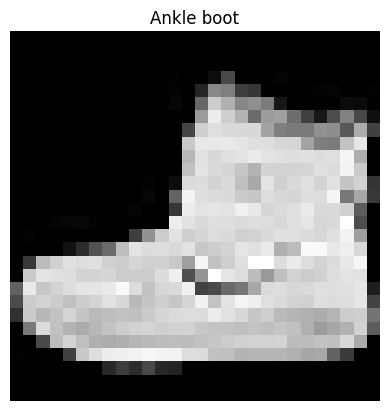
# Plot more images
torch.manual_seed(42)

fig=plt.figure(figsize=(9,9))
rows, cols = 4, 4
for i in range(1, rows*cols+1):
    random_idx = torch.randint(0, len(train_data), size=[1]).item()
    img, label = train_data[random_idx]
    fig.add_subplot(rows, cols, i)
    plt.imshow(img.squeeze(), cmap="gray")
    plt.title(class_names[label])
    plt.axis(False)
Do you think these items of closing (images) could be modelled with pure linear lines? Or do you think we'll need non-linearities?
2. Prepare DataLoader
Right now, our data is in the form of PyTorch Datasets.
DataLoader turns our dataset into a Python iterable
More specifically, we want to turn data into batches (or mini-batches).
Why would we do this?
- It is more computationally efficient, as in, your computer hardware may not be able to look (store in memory) at 60000 images in one hit. So we break it down to 32 images at a time (batch size of 32)
- It gives our neural network more chances to update its gradients per epoch.
train_data, test_data(Dataset FashionMNIST
Number of datapoints: 60000
Root location: data
Split: Train
StandardTransform
Transform: ToTensor(),
Dataset FashionMNIST
Number of datapoints: 10000
Root location: data
Split: Test
StandardTransform
Transform: ToTensor())from torch.utils.data import DataLoader
# Setup the batch size hyperparameter
BATCH_SIZE = 32
# Turn datasets into iterables (batches)
train_dataloader = DataLoader(
dataset=train_data,
batch_size=BATCH_SIZE,
shuffle=True
)
test_dataloader = DataLoader(
dataset=test_data,
batch_size=BATCH_SIZE,
shuffle=False
)
train_dataloader, test_dataloader(<torch.utils.data.dataloader.DataLoader at 0x7e1fa818a5c0>,
<torch.utils.data.dataloader.DataLoader at 0x7e1fa818b0d0>)# Let's check out what we've created
print(f"DataLoaders: {train_dataloader, test_dataloader}")
print(f"Length of train_dataloader: {len(train_dataloader)} batches of {BATCH_SIZE}")
print(f"Length of test_dataloader: {len(test_dataloader)} of batch size {BATCH_SIZE}")DataLoaders: (<torch.utils.data.dataloader.DataLoader object at 0x7e1fa818a5c0>, <torch.utils.data.dataloader.DataLoader object at 0x7e1fa818b0d0>)
Length of train_dataloader: 1875 batches of 32
Length of test_dataloader: 313 of batch size 32
train_features_batch, train_labels_batch = next(iter(train_dataloader))
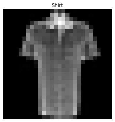
train_features_batch.shape, train_labels_batch.shape(torch.Size([32, 1, 28, 28]), torch.Size([32]))# Show a sample
torch.manual_seed(42)
random_idx = torch.randint(0, len(train_features_batch), size=[1]).item()
img, label = train_features_batch[random_idx], train_labels_batch[random_idx]
plt.imshow(img.squeeze(), cmap="gray")
plt.title(class_names[label])
plt.axis(False)
print(f"Image size: {img.shape}")
print(f"Label: {label}, label size: {label.shape}")Image size: torch.Size([1, 28, 28])
Label: 6, label size: torch.Size([])
3. Model 0. Build a baseline model
When starting to build a series of machine learning experiments, it's best practise to start with a baseline model
A baseline model is a simple model you will try and improve upon with subsequent model/experiments.
In other words: start simply and add complexity when necessary
# Create a flatten layer
flatten_model = nn.Flatten()

# Get a single sample
x = train_features_batch[0]

# Flatten the sample
output = flatten_model(x) # perform forward pass

# Print out what happened
print(f"Shape before flattening: {x.shape} -> [color_channels, height, width]")
print(f"Shape after flattening: {output.shape} -> [color_channels, height*width]")
Shape before flattening: torch.Size([1, 28, 28]) -> [color_channels, height, width]
Shape after flattening: torch.Size([1, 784]) -> [color_channels, height*width]
from torch import nn

class FashionMNISTModelV0(nn.Module):
    def __init__(
        self,
        input_shape: int,
        hidden_units: int,
        output_shape: int
    ):
        super().__init__()
        self.layer_stack = nn.Sequential(
            nn.Flatten(),
            nn.Linear(in_features=input_shape, out_features=hidden_units),
            nn.Linear(in_features=hidden_units, out_features=output_shape)
        )

    def forward(self, x):
return self.layer_stack(x)torch.manual_seed(42)
# Setup model with input parameters
model_0 = FashionMNISTModelV0(
input_shape=784,
hidden_units=10,
output_shape=len(class_names)
).to("cpu")
model_0FashionMNISTModelV0(
(layer_stack): Sequential(
(0): Flatten(start_dim=1, end_dim=-1)
(1): Linear(in_features=784, out_features=10, bias=True)
(2): Linear(in_features=10, out_features=10, bias=True)
)
)dummy_x = torch.rand([1, 1, 28, 28])
model_0(dummy_x)tensor([[-0.0315, 0.3171, 0.0531, -0.2525, 0.5959, 0.2112, 0.3233, 0.2694,
-0.1004, 0.0157]], grad_fn=<AddmmBackward0>)3.1 Setup loss, otimizer and evaluation metrics
- Loss function - since we're working with multi-class data, our loss
function will be
nn.CrossEntropyLoss() - Optimizer - our optimizer
torch.optim.SGD()(stochastic gradient descent) - Evaluation metric - since we're working on a classification problem, let's use accuracy as our evaluation metric
import requests
from pathlib import Path

# Download helper functions from Learn Pytorch repo
if Path("helper_functions.py").is_file():
    print("already exists")
else:
    print("downloading file")
    request = requests.get("https://raw.githubusercontent.com/mrdbourke/pytorch-deep-learning/main/helper_functions.py")
    with open("helper_functions.py", "wb") as f:
        f.write(request.content)
downloading file
# Import accuracy metric
from helper_functions import accuracy_fn

# Setup loss function and optimizer
loss_fn = nn.CrossEntropyLoss()
optimizer = torch.optim.SGD(params=model_0.parameters(), lr=0.1)
3.2 Create a function to time our experiments
Machine learning is very experimental.
Two of the main things you'll often want to track are:
- Model's performance (loss and accuracy values etc)
- How fast it runs
from timeit import default_timer as timer

def print_train_time(start: float, end: float, device: torch.device = None):
    """
    Prints difference between start and end time
    """

    total_time = end - start
    print(f"Train time on {device}: {total_time:.3f} seconds")
    return total_time
start_time = timer()
end_time = timer()
print_train_time(start=start_time, end=end_time, device="cpu")Train time on cpu: 0.000 seconds
2.6355000045441557e-053.3 Creating a training loop and training a model on batches of data
- Loop through epochs.
- Loop through training batches, perform training steps, calculate the training loss per batch.
- Loop through testing batches, perform testing steps, claculate the test loss per batch
- Print out what's happening
- Time it all (for fun)
# Import tqdm for progress bar
from tqdm.auto import tqdm

# Set the seed and start the timer
torch.manual_seed(42)
train_time_start_on_cpu = timer()

# Set the number of epochs (we'll keep it small for faster training loop)
epochs = 3

# Create training and test loop
for epoch in tqdm(range(epochs)):
    print(f"Epoch: {epoch}\n------")
    # Training
    train_loss = 0

    # Add a loop to loop through the training batches
    for batch, (X, y) in enumerate(train_dataloader):
        model_0.train()
        # 1. Forward pass
        y_pred = model_0(X)

        # 2. Calculate the loss
        loss = loss_fn(y_pred, y)
        train_loss += loss # accumulate train loss

        # 3. Optimizer zero grad
        optimizer.zero_grad()

        # 4. Loss bachward
        loss.backward()

        # 5. Optimizer step
        optimizer.step()

        # Print out what's happening
        if batch % 400 == 0:
            print(f"Looked at {batch * len(X)}/{len(train_dataloader.dataset)} examples")

    # Devide total train loss by length of train dataloader
    train_loss /= len(train_dataloader)

    ### Testing
    test_loss, test_acc = 0, 0
    model_0.eval()
    with torch.inference_mode():
        for X_test, y_test in test_dataloader:
            # 1. froward pass
            test_pred = model_0(X_test)

            # 2. Calculate the loss (accumulatevly)
            test_loss += loss_fn(test_pred, y_test)

            # 3. Calculate accuracy
            test_acc += accuracy_fn(y_true=y_test, y_pred=test_pred.argmax(dim=1))

        # Calculate the test loss average per batch
        test_loss /= len(test_dataloader)

        # Calculate the test acc average per batch
        test_acc /= len(test_dataloader)

    # Print out what's happening
    print(f"\nTrain loss: {train_loss:.4f} | test loss: {test_loss:.4f} | test accuracy: {test_acc:.2f}")

# Calculate train time
train_time_end_on_cpu = timer()
total_train_time_model_0 = print_train_time(
    start=train_time_start_on_cpu,
    end=train_time_end_on_cpu,
    device=str(next(model_0.parameters()).device)
){"model_id":"975bdc5c00264619829c79525eaa6d78","version_major":2,"version_minor":0}Epoch: 0
------
Looked at 0/60000 examples
Looked at 12800/60000 examples
Looked at 25600/60000 examples
Looked at 38400/60000 examples
Looked at 51200/60000 examples
Train loss: 0.5904 | test loss: 0.5095 | test accuracy: 82.04
Epoch: 1
Looked at 0/60000 examples
Looked at 12800/60000 examples
Looked at 25600/60000 examples
Looked at 38400/60000 examples
Looked at 51200/60000 examples
Train loss: 0.4763 | test loss: 0.4799 | test accuracy: 83.20
Epoch: 2
Looked at 0/60000 examples
Looked at 12800/60000 examples
Looked at 25600/60000 examples
Looked at 38400/60000 examples
Looked at 51200/60000 examples
Train loss: 0.4550 | test loss: 0.4766 | test accuracy: 83.43
Train time on cpu: 29.723 seconds
4. Make predictions and get Model 0 results
torch.manual_seed(42)
def eval_model(model: torch.nn.Module,
              data_loader: torch.utils.data.DataLoader,
              loss_fn: torch.nn.Module,
              accuracy_fn,
              device = "cpu"):
    """
    Returns a dictionary containing the results of model predicting on data_loader
    """

    loss, acc = 0, 0
    model.eval()
    with torch.inference_mode():
        for X, y in tqdm(data_loader):
            # Make our data device agnostic
            X, y = X.to(device), y.to(device)
            # Make predictions
            y_pred = model(X)

            # Accumulate the loss and acc values per batch
            loss += loss_fn(y_pred, y)
            acc += accuracy_fn(y_true=y,
                              y_pred=y_pred.argmax(dim=1))

        #Scale loss and acc to find the average loss/acc per batch
        loss /= len(data_loader)
        acc /= len(data_loader)

    return {"model_name": model.__class__.__name__,
            "model_loss": loss.item(),
            "model_acc": acc}

# Calculate model 0 results on test dataset
model_0_results = eval_model(model=model_0,
                            data_loader=test_dataloader,
                            loss_fn=loss_fn,
                            accuracy_fn=accuracy_fn,
                            device="cpu")
model_0_results{"model_id":"edb7f60a1161425eb01c5c6d8b1c9da7","version_major":2,"version_minor":0}{'model_name': 'FashionMNISTModelV0',
'model_loss': 0.47663894295692444,
'model_acc': 83.42651757188499}5. Setup device agnostic-code (for using a GPU if there is one)
device = "cuda" if torch.cuda.is_available() else "cpu"
device'cuda'6. Model 1: Building a better model with non-linearity
We learned about the power of non-linearity
# Create a model with linear and non-linear layers
class FashionMNISTModelV1(nn.Module):
    def __init__(self,
                input_shape: int,
                hidden_units: int,
                output_shape: int):
        super().__init__()
        self.layer_stack = nn.Sequential(
            nn.Flatten(), # Flatten input into a single vector
            nn.Linear(in_features=input_shape, out_features=hidden_units),
            nn.ReLU(),
            nn.Linear(in_features=hidden_units, out_features=hidden_units),
            nn.ReLU(),
            nn.Linear(in_features=hidden_units, out_features=output_shape)
        )

    def forward(self, x):
return self.layer_stack(x)device'cuda'!nvidia-smiTue Jul 9 15:28:06 2024
+-----------------------------------------------------------------------------------------+
| NVIDIA-SMI 550.90.07 Driver Version: 550.90.07 CUDA Version: 12.4 |
|-----------------------------------------+------------------------+----------------------+
| GPU Name Persistence-M | Bus-Id Disp.A | Volatile Uncorr. ECC |
| Fan Temp Perf Pwr:Usage/Cap | Memory-Usage | GPU-Util Compute M. |
| | | MIG M. |
|=========================================+========================+======================|
| 0 Tesla T4 Off | 00000000:00:04.0 Off | 0 |
| N/A 48C P8 12W / 70W | 3MiB / 15360MiB | 0% Default |
| | | N/A |
+-----------------------------------------+------------------------+----------------------+
| 1 Tesla T4 Off | 00000000:00:05.0 Off | 0 |
| N/A 51C P8 11W / 70W | 3MiB / 15360MiB | 0% Default |
| | | N/A |
+-----------------------------------------+------------------------+----------------------+
+-----------------------------------------------------------------------------------------+
| Processes: |
| GPU GI CI PID Type Process name GPU Memory |
| ID ID Usage |
|=========================================================================================|
| No running processes found |
+-----------------------------------------------------------------------------------------+
# Create an instance of model
model_1 = FashionMNISTModelV1(input_shape=28*28,
                             hidden_units=30,
                             output_shape=len(class_names)).to(device)

model_1
FashionMNISTModelV1(
(layer_stack): Sequential(
(0): Flatten(start_dim=1, end_dim=-1)
(1): Linear(in_features=784, out_features=30, bias=True)
(2): ReLU()
(3): Linear(in_features=30, out_features=30, bias=True)
(4): ReLU()
(5): Linear(in_features=30, out_features=10, bias=True)
)
)next(model_1.parameters()).devicedevice(type='cuda', index=0)next(model_0.parameters()).devicedevice(type='cpu')6.1 Setup loss, optimizer and evaluation metrics
from helper_functions import accuracy_fn
loss_fn = nn.CrossEntropyLoss()
optimizer = torch.optim.SGD(params=model_1.parameters(), lr=0.1)
6.2 Functionazing training and evaluation/testing loops
Let's create a function for:
- training loop -
train_step() - testing loop -
test_step()
def train_step(model: torch.nn.Module,
               data_loader: torch.utils.data.DataLoader,
               loss_fn: torch.nn.Module,
               optimizer: torch.optim.Optimizer,
               accuracy_fn,
               device: torch.device = device):
    """
    Performs a training with model trying to learn a data_loader
    """
    # Training
    train_loss, train_acc = 0, 0

    # Put model into training mode
    model.train()

    # Add a loop to loop through the training batches
    for batch, (X, y) in enumerate(data_loader):
        # Put data on target device
        X, y = X.to(device), y.to(device)

        # 1. Forward pass
        y_pred = model(X)

        # 2. Calculate the loss and accuracy
        loss = loss_fn(y_pred, y)
        train_loss += loss # accumulate train loss
        train_acc += accuracy_fn(y_true=y, y_pred=y_pred.argmax(dim=1))

        # 3. Optimizer zero grad
        optimizer.zero_grad()

        # 4. Loss bachward
        loss.backward()

        # 5. Optimizer step
        optimizer.step()

    # Devide total train loss and accuracy by length of train dataloader
    train_loss /= len(data_loader)
    train_acc /= len(data_loader)
    print(f"Train loss: {train_loss:.3f} | Train accuracy: {train_acc:.2f}%")


def test_step(model: torch.nn.Module,
               data_loader: torch.utils.data.DataLoader,
               loss_fn: torch.nn.Module,
               accuracy_fn,
               device: torch.device = device):
    """
    Performs a testing with data_loader trying to evaluate the model
    """
    # Training
    test_loss, test_acc = 0, 0

    # Put model into testing mode
    model.eval()

    # Turn on inference mode context manager
    with torch.inference_mode():
        # Add a loop to loop through the training batches
        for X, y in data_loader:
            # Put data on target device
            X, y = X.to(device), y.to(device)

            # 1. Forward pass
            y_pred = model(X)

            # 2. Calculate the loss and accuracy
            loss = loss_fn(y_pred, y)
            test_loss += loss # accumulate train loss
            test_acc += accuracy_fn(y_true=y, y_pred=y_pred.argmax(dim=1))

        # Devide total train loss and accuracy by length of test dataloader
        test_loss /= len(data_loader)
        test_acc /= len(data_loader)
        print(f"Test loss: {test_loss:.3f} | Test accuracy: {test_acc:.2f}%\n")
# Import tqdm for progress bar
from tqdm.auto import tqdm
# Set the seed and start the timer
torch.manual_seed(42)
train_time_start_on_gpu = timer()
# Set the number of epochs (we'll keep it small for faster training loop)
epochs = 3
# Create training and test loop
for epoch in tqdm(range(epochs)):
print(f"Epoch: {epoch}\n------")
train_step(
model = model_1,
data_loader = train_dataloader,
loss_fn = loss_fn,
optimizer = optimizer,
accuracy_fn = accuracy_fn,
device = device
)
test_step(
model = model_1,
data_loader = test_dataloader,
loss_fn = loss_fn,
accuracy_fn = accuracy_fn,
device = device
)
# Calculate train time
train_time_end_on_gpu = timer()
total_train_time_model_1 = print_train_time(
start=train_time_start_on_gpu,
end=train_time_end_on_gpu,
device=str(next(model_1.parameters()).device)
){"model_id":"6d39c82dcf764aae8a2034637ebffa80","version_major":2,"version_minor":0}Epoch: 0
------
Train loss: 0.618 | Train accuracy: 77.49%
Test loss: 0.517 | Test accuracy: 81.36%
Epoch: 1
Train loss: 0.427 | Train accuracy: 84.23%
Test loss: 0.442 | Test accuracy: 84.05%
Epoch: 2
Train loss: 0.389 | Train accuracy: 85.66%
Test loss: 0.419 | Test accuracy: 84.49%
Train time on cuda:0: 31.800 seconds
model_0_results{'model_name': 'FashionMNISTModelV0',
'model_loss': 0.47663894295692444,
'model_acc': 83.42651757188499}Note: Sometimes , depending on your data/hardware you might find that your model trains faster on CPU than GPU.
Why is this?
- It could be that the overhead fro copying data/model to and from the GPU outweighs the compute benefits offered by the GPU.
- The hardware you're using has a better CPU in terms compute capabilities than the GPU
# Get model_1 results dictionary
model_1_results = eval_model(model=model_1,
                            data_loader=test_dataloader,
                            loss_fn=loss_fn,
                            accuracy_fn=accuracy_fn,
                            device=device)
model_1_results{"model_id":"5f1ffe01f1054d8db65eda9b8185b32d","version_major":2,"version_minor":0}{'model_name': 'FashionMNISTModelV1',
'model_loss': 0.4194523096084595,
'model_acc': 84.49480830670926}model_0_results{'model_name': 'FashionMNISTModelV0',
'model_loss': 0.47663894295692444,
'model_acc': 83.42651757188499}Model 2: Building a Convolutional Neural Network (CNN)
CNN's are also known ConvNets.
CNN's are known for their capabilities to find patterns in visual data
# Create a convolutional neural network

class FashionMNISTModelV2(nn.Module):
    """
    Model architecture that replicates the TinyVGG
    model from CNN explainer website
    """

    def __init__(self, input_shape: int,
                hidden_units: int,
                output_shape: int):
        super().__init__()
        self.conv_block_1 = nn.Sequential(
            # Create a conv layer
            nn.Conv2d(in_channels = input_shape,
                      out_channels= hidden_units,
                     kernel_size=3,
                     stride=1,
                     padding=1), # values we can set ourselves in our NN's are called hyperparameters
            nn.ReLU(),
            nn.Conv2d(in_channels=hidden_units,
                     out_channels=hidden_units,
                     kernel_size=3,
                     stride=1,
                     padding=1),
            nn.ReLU(),
            nn.MaxPool2d(kernel_size=2)
        )
        self.conv_block_2 = nn.Sequential(
            nn.Conv2d(in_channels=hidden_units,
                     out_channels=hidden_units,
                     kernel_size=3,
                     stride=1,
                     padding=1),
            nn.ReLU(),
            nn.Conv2d(in_channels=hidden_units,
                     out_channels=hidden_units,
                     kernel_size=3,
                     stride=1,
                     padding=1),
            nn.ReLU(),
            nn.MaxPool2d(kernel_size=2)
        )
        self.classifier = nn.Sequential(
            nn.Flatten(),
            nn.Linear(in_features=hidden_units*7*7, # there is a trick to calculate this
                     out_features=output_shape)
        )

    def forward(self, x):
        x = self.conv_block_1(x)
        #print(x.shape)
        x = self.conv_block_2(x)
        #print(x.shape)
        x = self.classifier(x)
        #print(x.shape)
return xtorch.manual_seed(42)
model_2 = FashionMNISTModelV2(input_shape=1,
hidden_units=10,
output_shape=len(class_names)).to(device)
model_2FashionMNISTModelV2(
(conv_block_1): Sequential(
(0): Conv2d(1, 10, kernel_size=(3, 3), stride=(1, 1), padding=(1, 1))
(1): ReLU()
(2): Conv2d(10, 10, kernel_size=(3, 3), stride=(1, 1), padding=(1, 1))
(3): ReLU()
(4): MaxPool2d(kernel_size=2, stride=2, padding=0, dilation=1, ceil_mode=False)
)
(conv_block_2): Sequential(
(0): Conv2d(10, 10, kernel_size=(3, 3), stride=(1, 1), padding=(1, 1))
(1): ReLU()
(2): Conv2d(10, 10, kernel_size=(3, 3), stride=(1, 1), padding=(1, 1))
(3): ReLU()
(4): MaxPool2d(kernel_size=2, stride=2, padding=0, dilation=1, ceil_mode=False)
)
(classifier): Sequential(
(0): Flatten(start_dim=1, end_dim=-1)
(1): Linear(in_features=490, out_features=10, bias=True)
)
)plt.imshow(image.squeeze(), cmap="gray")<matplotlib.image.AxesImage at 0x7e1fa81a1cf0>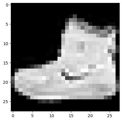
rand_mage_tensor = torch.randn(size=(1, 28, 28)).to(device)
# Pass image through model
model_2(rand_mage_tensor.unsqueeze(0))
tensor([[ 0.0366, -0.0940, 0.0686, -0.0485, 0.0068, 0.0290, 0.0132, 0.0084,
-0.0030, -0.0185]], device='cuda:0', grad_fn=<AddmmBackward0>)7.1 Stepping through
nn.Conv2d()
torch.manual_seed(42)

# Create a batch of images
images = torch.randn(size=(32, 3, 64, 64))
test_image = images[0]

print(f"Image batch shape: {images.shape}")
print(f"Single image shape: {test_image.shape}")
Image batch shape: torch.Size([32, 3, 64, 64])
Single image shape: torch.Size([3, 64, 64])
# Create a single conv2d layer
conv_layer = nn.Conv2d(in_channels=3,
                      out_channels=10,
                      kernel_size=(3,3),
                      stride=1,
                      padding=1)

# Pass the data through the convolutional layer
conv_output = conv_layer(test_image.unsqueeze(0))
conv_output.shape
torch.Size([1, 10, 64, 64])7.2 Stepping through
nn.MaxPool2d()
test_image.shapetorch.Size([3, 64, 64])# Print out the original image shape without unsqueeze dimension
print(f"Test image original shape: {test_image.shape}")
print(f"Test image with unsqueezed dimension: {test_image.unsqueeze(0).shape}")
# Create a sample nn.MaxPool2d layer
max_pool_layer = nn.MaxPool2d(kernel_size=2)
# Pass data through just the conv layer
tst_image_through_conv = conv_layer(test_image.unsqueeze(dim=0))
print(f"Shape after going through conv layer: {tst_image_through_conv.shape}")
# Pass data through the max pool layer
test_image_through_conv_and_max_pool = max_pool_layer(tst_image_through_conv)
print(f"Shape after going through conv layer and max pool layer: {test_image_through_conv_and_max_pool.shape}")Test image original shape: torch.Size([3, 64, 64])
Test image with unsqueezed dimension: torch.Size([1, 3, 64, 64])
Shape after going through conv layer: torch.Size([1, 10, 64, 64])
Shape after going through conv layer and max pool layer: torch.Size([1, 10, 32, 32])
torch.manual_seed(42)
# Create a random tensor with a similar number of dimensions to our image
random_tensor = torch.randn(size=(1, 1, 2, 2))
print(f"Original Tensor:\n {random_tensor}")
print(f"Original Tensor shape: {random_tensor.shape}")

# Create max pool layer
max_pool_layer = nn.MaxPool2d(kernel_size=2)

# Pass the random tensor through the max pool layer
random_tensor_through_max_pool = max_pool_layer(random_tensor)
print(f"Max pool tensor:\n {random_tensor_through_max_pool}")
print(f"Max pool tensor shape: {random_tensor_through_max_pool.shape}")
Original Tensor:
tensor([[[[0.3367, 0.1288],
[0.2345, 0.2303]]]])
Original Tensor shape: torch.Size([1, 1, 2, 2])
Max pool tensor:
tensor([[[[0.3367]]]])
Max pool tensor shape: torch.Size([1, 1, 1, 1])
7.3 Setup a
loss function and optimizer for model_2
# Setup loss function/eval metrics/optimizer
from helper_functions import accuracy_fn

loss_fn = nn.CrossEntropyLoss()
optimizer = torch.optim.SGD(params=model_2.parameters(), lr=0.1)
7.4 Training and testing model_2 using our training and test functions
torch.manual_seed(42)
torch.cuda.manual_seed(42)

# Measure time
from timeit import default_timer as timer
train_time_start_model_2 = timer()

# Train and test model
epochs = 3
for epoch in tqdm(range(epochs)):
    print(f"Epoch: {epoch}\n-------")
    train_step(model=model_2,
              data_loader=train_dataloader,
              loss_fn=loss_fn,
              optimizer=optimizer,
              accuracy_fn=accuracy_fn,
              device=device)
    test_step(model=model_2,
             data_loader=test_dataloader,
             loss_fn=loss_fn,
             accuracy_fn=accuracy_fn,
             device=device)

train_time_end_model_2 = timer()
total_train_time_model_2 = print_train_time(
    start=train_time_start_model_2,
    end=train_time_end_model_2,
    device=device
){"model_id":"3c88bb35c73844d68719b022110748a9","version_major":2,"version_minor":0}Epoch: 0
-------
Train loss: 0.588 | Train accuracy: 78.63%
Test loss: 0.405 | Test accuracy: 85.59%
Epoch: 1
Train loss: 0.364 | Train accuracy: 86.76%
Test loss: 0.351 | Test accuracy: 87.11%
Epoch: 2
Train loss: 0.326 | Train accuracy: 88.16%
Test loss: 0.321 | Test accuracy: 88.63%
Train time on cuda: 36.717 seconds
# Get model_2 results
model_2_results = eval_model(model=model_2,
                            data_loader=test_dataloader,
                            loss_fn=loss_fn,
                            accuracy_fn=accuracy_fn,
                            device=device)
model_2_results{"model_id":"fc046fe4e0174802a7e03b85066f0a3d","version_major":2,"version_minor":0}{'model_name': 'FashionMNISTModelV2',
'model_loss': 0.32091188430786133,
'model_acc': 88.62819488817891}8. Compare model results and training time
import pandas as pd
compare_results = pd.DataFrame([model_0_results,
                               model_1_results,
                               model_2_results])
compare_results| model_name | model_loss | model_acc | |
|---|---|---|---|
| 0 | FashionMNISTModelV0 | 0.476639 | 83.426518 |
| 1 | FashionMNISTModelV1 | 0.419452 | 84.494808 |
| 2 | FashionMNISTModelV2 | 0.320912 | 88.628195 |
# Add training time to results comparison
compare_results["training_time"] = [total_train_time_model_0,
                                   total_train_time_model_1,
                                   total_train_time_model_2]
compare_results| model_name | model_loss | model_acc | training_time | |
|---|---|---|---|---|
| 0 | FashionMNISTModelV0 | 0.476639 | 83.426518 | 29.722932 |
| 1 | FashionMNISTModelV1 | 0.419452 | 84.494808 | 31.799669 |
| 2 | FashionMNISTModelV2 | 0.320912 | 88.628195 | 36.716990 |
# Visualize our model results
compare_results.set_index("model_name")["model_acc"].plot(kind="barh")
plt.xlabel("accuracy %")
plt.ylabel("model")
Text(0, 0.5, 'model')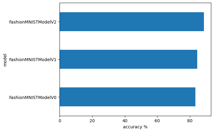
9. Make and evaluate random predictions with best model
def make_predictions(model: torch.nn.Module,
                    data: list,
                    device: torch.device = device):
    pred_probs = []
    model.to(device)
    model.eval()
    with torch.inference_mode():
        for sample in data:
            # Prepare the sample (add a batch dimension and pass to target device)
            sample = torch.unsqueeze(sample, dim=1).to(device)

            # Forward pass (model output row logits)
            pred_logits = model(sample)

            # Get prediction pobability (logit -> prediction probabilities)
            pred_prob = torch.softmax(pred_logits.squeeze(), dim=0)

            # Get pred_prob off the GPU for futher calculations
            pred_probs.append(pred_prob.cpu())

    # Stack the pred probs to turn list into tensor
    return torch.stack(pred_probs)
import random
#random.seed(42)
test_samples = []
test_labels = []
for sample, label in random.sample(list(test_data), k=9):
test_samples.append(sample)
test_labels.append(label)
# View the first sample shape
test_samples[0].shapetorch.Size([1, 28, 28])plt.imshow(test_samples[0].squeeze(), cmap="gray")
plt.title(class_names[test_labels[0]])Text(0.5, 1.0, 'Coat')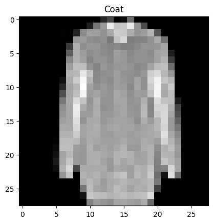
# Make predictions
pred_probs = make_predictions(model=model_2,
                             data=test_samples)

# View first two prediction probablities
pred_probs[:2]
tensor([[2.1653e-02, 5.4951e-04, 5.8419e-02, 4.8616e-02, 4.7800e-01, 6.3986e-05,
3.7636e-01, 2.1623e-05, 1.6141e-02, 1.7873e-04],
[4.1643e-01, 8.5945e-05, 4.0930e-03, 1.5850e-02, 5.2843e-05, 5.5267e-07,
5.6329e-01, 2.4754e-07, 2.0591e-04, 7.7119e-07]])# Convert prediction probabilities to labels
pred_classes = pred_probs.argmax(dim=1)
pred_classestensor([4, 6, 1, 9, 9, 0, 0, 4, 9])test_labels[4, 0, 1, 9, 9, 0, 0, 4, 9]# Plot predictions
plt.figure(figsize=(9, 9))
nrows = 3
ncols = 3
for i, sample in enumerate(test_samples):
# Create subplot
plt.subplot(nrows, ncols, i+1)
# Plot the target image
plt.imshow(sample.squeeze(), cmap="gray")
# Find the prediction (in text form e.g "Sandal")
pred_label = class_names[pred_classes[i]]
# Get the truth label (in text form)
truth_label = class_names[test_labels[i]]
# Create a title for the plot
title_text = f"Pred: {pred_label} | Truth: {truth_label}"
# Check for equality between pred and truth and change color of title text
if pred_label == truth_label:
plt.title(title_text, fontsize=10, c="g")
else:
plt.title(title_text, fontsize=10, c="r")
plt.axis(False)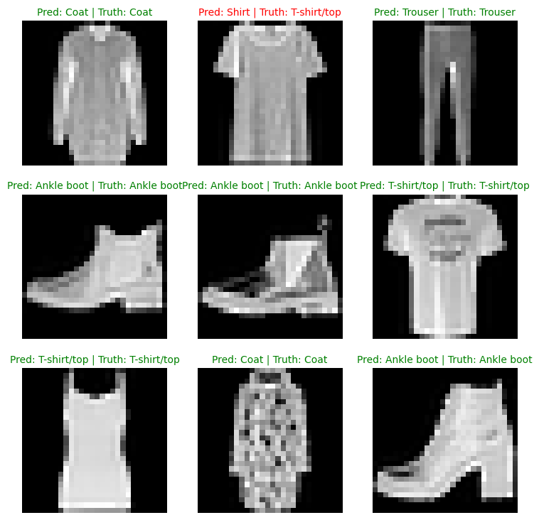
10. Making a confusion matrix for futher prediction evaluation
A confusion matrix is a fantastic way of evaluating your classification models visually
- Make predictions with our trained model on the test dataset
- Make a confusion matrix
torchmetrics.ConfusionMatrix - Plot the confusion matrix using
mlxtend.plotting.plot_confusion_matrix()
from tqdm.auto import tqdm

# 1. Make predictions with trained model
y_preds = []
model_2.eval()
with torch.inference_mode():
    for X, y in tqdm(test_dataloader, desc="Making predictions..."):
        # Send the data and targets to target device
        X, y = X.to(device), y.to(device)

        # Do the forward pass
        y_logit = model_2(X)

        # Turn predictions from logits -> prediction probabilities -> prediction labels
        y_pred = torch.softmax(y_logit.squeeze(), dim=0).argmax(dim=1)

        # Put predictions on cpu for evaluations
        y_preds.append(y_pred.cpu())

# Concatenate list of predictions into tensor
print(y_preds[0].shape)
y_pred_tensor = torch.cat(y_preds)
print(y_pred_tensor.shape)
y_pred_tensor[:10]{"model_id":"86b057e1b4044e849ebebcdf4418e22a","version_major":2,"version_minor":0}torch.Size([32])
torch.Size([10000])
tensor([9, 2, 1, 1, 6, 1, 4, 6, 5, 7])import torchmetrics, mlxtend
print(f"mlxtend version: {mlxtend.__version__}")
assert int(mlxtend.__version__.split(".")[1]) >= 19, "mlxtend version should be 0.19.0 or higher"mlxtend version: 0.23.1
from torchmetrics import ConfusionMatrix
from mlxtend.plotting import plot_confusion_matrix

# 2. Setup confusion instance and compare predictions to targets
confmat = ConfusionMatrix(task='multiclass', num_classes=len(class_names))
confmat_tensor = confmat(preds=y_pred_tensor,
                        target=test_data.targets)

# 3. Plot the confusion matrix
fig, ax = plot_confusion_matrix(
    conf_mat=confmat_tensor.numpy(), # matplotlib likes working with numpy
    class_names=class_names,
    figsize=(10, 7)
)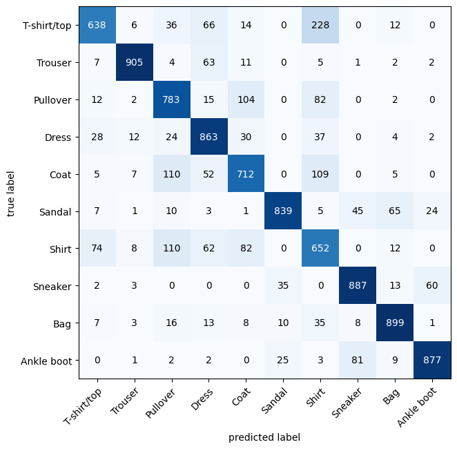
confmat_tensortensor([[638, 6, 36, 66, 14, 0, 228, 0, 12, 0],
[ 7, 905, 4, 63, 11, 0, 5, 1, 2, 2],
[ 12, 2, 783, 15, 104, 0, 82, 0, 2, 0],
[ 28, 12, 24, 863, 30, 0, 37, 0, 4, 2],
[ 5, 7, 110, 52, 712, 0, 109, 0, 5, 0],
[ 7, 1, 10, 3, 1, 839, 5, 45, 65, 24],
[ 74, 8, 110, 62, 82, 0, 652, 0, 12, 0],
[ 2, 3, 0, 0, 0, 35, 0, 887, 13, 60],
[ 7, 3, 16, 13, 8, 10, 35, 8, 899, 1],
[ 0, 1, 2, 2, 0, 25, 3, 81, 9, 877]])11. Save and load best performing model
from pathlib import Path

# Create model directory path
MODEL_PATH = Path("models")
MODEL_PATH.mkdir(parents=True,
                exist_ok=True)

# Create model save
MODEL_NAME = "03_pytorch_computer_vision_model_2.pth"
MODEL_SAVE_PATH = MODEL_PATH / MODEL_NAME
MODEL_SAVE_PATHPosixPath('models/03_pytorch_computer_vision_model_2.pth')# Save the model state dict
torch.save(obj=model_2.state_dict(), f=MODEL_SAVE_PATH)# Create new instance
torch.manual_seed(42)
loaded_model_2 = FashionMNISTModelV2(input_shape=1,
hidden_units=10,
output_shape=len(class_names))
# Load in the save state_dict()
loaded_model_2.load_state_dict(torch.load(f=MODEL_SAVE_PATH))
loaded_model_2 = loaded_model_2.to(device)model_2_results{'model_name': 'FashionMNISTModelV2',
'model_loss': 0.32091188430786133,
'model_acc': 88.62819488817891}# Evaluate loaded model
torch.manual_seed(42)
loaded_model_2_results = eval_model(
model=loaded_model_2,
data_loader=test_dataloader,
loss_fn=loss_fn,
accuracy_fn=accuracy_fn,
device=device
)
loaded_model_2_results{"model_id":"74e519b540274321a81c0886ea5fc673","version_major":2,"version_minor":0}{'model_name': 'FashionMNISTModelV2',
'model_loss': 0.32091188430786133,
'model_acc': 88.62819488817891}# Check if model results are close to each other
torch.isclose(torch.tensor(model_2_results["model_loss"]),
torch.tensor(loaded_model_2_results["model_loss"]),
atol=1e-02) # tollerancetensor(True)- Q: What are 3 areas in industry where computer vision is currently being used?
A: Computer vision is making significant contributions across a wide range of industries. Here are several key areas where it is currently being utilized:
- Healthcare:
- Medical Imaging and Diagnostics: Enhancing the analysis of X-rays, MRIs, and CT scans for early disease detection.
- Surgical Assistance: Providing real-time imaging and augmented reality overlays during surgeries.
- Telemedicine: Enabling remote patient monitoring through analysis of images and videos.
- Retail:
- Automated Checkout Systems: Implementing cashier-less shopping experiences with real-time product tracking.
- Inventory Management: Monitoring stock levels and managing inventory through shelf image analysis.
- Customer Behavior Analysis: Tracking customer movements and interactions to optimize store layouts and product placements.
- Manufacturing:
- Quality Control: Inspecting products for defects and ensuring high-quality standards on production lines.
- Predictive Maintenance: Analyzing machinery images to predict maintenance needs and prevent breakdowns.
- Automation and Robotics: Enhancing the capabilities of industrial robots through vision-based guidance and inspection.
- Automotive:
- Autonomous Vehicles: Enabling self-driving cars to navigate and understand their surroundings.
- Driver Assistance Systems: Providing features like lane departure warnings, pedestrian detection, and adaptive cruise control.
- Vehicle Inspection: Automating the inspection process for manufacturing and maintenance.
- Security and Surveillance:
- Facial Recognition: Identifying individuals for security and authentication purposes.
- Behavior Analysis: Monitoring and analyzing behavior patterns to detect suspicious activities.
- Access Control: Managing entry to secure areas through visual identification.
- Agriculture:
- Crop Monitoring: Using drones and cameras to monitor crop health, identify diseases, and optimize irrigation.
- Livestock Management: Tracking the health and movement of animals to improve farming practices.
- Yield Prediction: Analyzing images to predict crop yields and optimize harvest timing.
- Finance and Banking:
- Fraud Detection: Using visual data to detect fraudulent activities at ATMs and during transactions.
- Customer Service: Implementing facial recognition for secure access to banking services.
- Document Processing: Automating the processing of checks and other financial documents through image analysis.
- Entertainment and Media:
- Content Creation and Editing: Enhancing video production with special effects, automated editing, and scene recognition.
- Personalization: Tailoring content recommendations based on visual analysis of user preferences.
- Interactive Experiences: Creating augmented and virtual reality experiences.
- Live information. When you walk, your device finds qr codes and get information about what it sees. When you ask a question, it replies you with information it collected.
- Search "what is overfitting in machine learning" and write down a sentence about what you find.
A: Training data always contains noise. Overfitting is when model start to focus too much on noise and missing real pattern. Then the train loss goes down, but test loss goes up. But, if there are a lot of data, at some point model might understand this is a noise and loss will go down on testing as well. This is called grokking
- Search "ways to prevent overfitting in machine learning", write down 3 of the things you find and a sentence about each. Note: there are lots of these, so don't worry too much about all of them, just pick 3 and start with those.
- Cross-Validation: Cross-validation is a technique where the training data is split into multiple subsets (folds). The model is trained and validated multiple times, each time using a different subset for validation and the remaining subsets for training. This helps in ensuring that the model’s performance is consistent across different subsets of data and not just tailored to a particular subset, thus reducing overfitting. Common methods include k-fold cross-validation and leave-one-out cross-validation.
- Early Stopping: During the training process, the model’s performance is monitored on a validation dataset after each iteration. Early stopping involves halting the training process when the model’s performance on the validation set stops improving, even if it continues to improve on the training set. This prevents the model from learning the noise and irrelevant patterns in the training data, which can lead to overfitting.
- Data Augmentation: Data augmentation artificially increases the size of the training dataset by generating new data points from the existing data. This can be done through techniques like rotating, flipping, and cropping images in image datasets or using methods like back-translation and noise addition in text data. Data augmentation enhances the diversity of the training data, helping the model learn more robust and generalizable features, thus reducing overfitting.
- Load the torchvision.datasets.MNIST() train and test datasets.
import torchvision
from torchvision import datasets
from torchvision.transforms import ToTensor
mnist_train = datasets.MNIST(
root="data_mnist",
train=True,
download=True,
transform=ToTensor(),
target_transform=None
)
mnist_test = datasets.MNIST(
root="data_mnist",
train=False,
download=True,
transform=ToTensor(),
target_transform=None
)
len(mnist_train), len(mnist_test)Downloading http://yann.lecun.com/exdb/mnist/train-images-idx3-ubyte.gz
Failed to download (trying next):
HTTP Error 403: Forbidden
Downloading https://ossci-datasets.s3.amazonaws.com/mnist/train-images-idx3-ubyte.gz
Downloading https://ossci-datasets.s3.amazonaws.com/mnist/train-images-idx3-ubyte.gz to data_mnist/MNIST/raw/train-images-idx3-ubyte.gz
100%|██████████| 9912422/9912422 [00:00<00:00, 35317727.75it/s]
Extracting data_mnist/MNIST/raw/train-images-idx3-ubyte.gz to data_mnist/MNIST/raw
Downloading http://yann.lecun.com/exdb/mnist/train-labels-idx1-ubyte.gz
Failed to download (trying next):
HTTP Error 403: Forbidden
Downloading https://ossci-datasets.s3.amazonaws.com/mnist/train-labels-idx1-ubyte.gz
Downloading https://ossci-datasets.s3.amazonaws.com/mnist/train-labels-idx1-ubyte.gz to data_mnist/MNIST/raw/train-labels-idx1-ubyte.gz
100%|██████████| 28881/28881 [00:00<00:00, 1031793.85it/s]
Extracting data_mnist/MNIST/raw/train-labels-idx1-ubyte.gz to data_mnist/MNIST/raw
Downloading http://yann.lecun.com/exdb/mnist/t10k-images-idx3-ubyte.gz
Failed to download (trying next):
HTTP Error 403: Forbidden
Downloading https://ossci-datasets.s3.amazonaws.com/mnist/t10k-images-idx3-ubyte.gz
Downloading https://ossci-datasets.s3.amazonaws.com/mnist/t10k-images-idx3-ubyte.gz to data_mnist/MNIST/raw/t10k-images-idx3-ubyte.gz
100%|██████████| 1648877/1648877 [00:00<00:00, 10376944.99it/s]
Extracting data_mnist/MNIST/raw/t10k-images-idx3-ubyte.gz to data_mnist/MNIST/raw
Downloading http://yann.lecun.com/exdb/mnist/t10k-labels-idx1-ubyte.gz
Failed to download (trying next):
HTTP Error 403: Forbidden
Downloading https://ossci-datasets.s3.amazonaws.com/mnist/t10k-labels-idx1-ubyte.gz
Downloading https://ossci-datasets.s3.amazonaws.com/mnist/t10k-labels-idx1-ubyte.gz to data_mnist/MNIST/raw/t10k-labels-idx1-ubyte.gz
100%|██████████| 4542/4542 [00:00<00:00, 2462899.65it/s]Extracting data_mnist/MNIST/raw/t10k-labels-idx1-ubyte.gz to data_mnist/MNIST/raw
(60000, 10000)- Visualize at least 5 different samples of the MNIST training dataset.
import matplotlib.pyplot as plt
import torch
n_row = 1
n_col = 5
_, axs = plt.subplots(n_row, n_col, figsize=(12, 12))
axs = axs.flatten()
for i, ax in zip(range(5), axs):
random_train_number = torch.randint(low=0, high=len(mnist_train), size=()).item()
image, label = mnist_train[random_train_number]
ax.imshow(image.squeeze(), cmap="gray")
ax.set_title(f"Number {label}")
plt.show()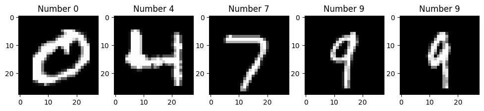
- Turn the MNIST train and test datasets into dataloaders using torch.utils.data.DataLoader, set the batch_size=32.
from torch.utils.data import DataLoadertrain_dataloader = DataLoader(mnist_train,
batch_size=32,
shuffle=True)
test_dataloader = DataLoader(mnist_test,
batch_size=32,
shuffle=False)
len(train_dataloader), len(test_dataloader), mnist_train.classes(1875,
313,
['0 - zero',
'1 - one',
'2 - two',
'3 - three',
'4 - four',
'5 - five',
'6 - six',
'7 - seven',
'8 - eight',
'9 - nine'])- Recreate model_2 used in this notebook (the same model from the CNN Explainer website, also known as TinyVGG) capable of fitting on the MNIST dataset.
from torch import nn

class MNISTModel(nn.Module):
    def __init__(self):
        super().__init__()
        self.layer_1 = nn.Sequential(
            nn.Conv2d(in_channels=1,
                     out_channels=10,
                     kernel_size=3,
                     stride=1,
                     padding=1),
            nn.ReLU(),
            nn.Conv2d(in_channels=10,
                     out_channels=10,
                     kernel_size=3,
                     stride=1,
                     padding=1),
            nn.ReLU(),
            nn.MaxPool2d(kernel_size=2)
        )
        self.layer_2 = nn.Sequential(
            nn.Conv2d(in_channels=10,
                     out_channels=10,
                     kernel_size=3,
                     stride=1,
                     padding=1),
            nn.ReLU(),
            nn.Conv2d(in_channels=10,
                     out_channels=10,
                     kernel_size=3,
                     stride=1,
                     padding=1),
            nn.ReLU(),
            nn.MaxPool2d(kernel_size=2)
        )
        self.classifier = nn.Sequential(
            nn.Flatten(),
            nn.Linear(in_features=10*7*7,
                     out_features=len(mnist_train.classes))
        )

    def forward(self, x):
        x = self.layer_1(x)
        x = self.layer_2(x)
        x = self.classifier(x)
        return x

model_e = MNISTModel().to("cuda")
model_e
MNISTModel(
(layer_1): Sequential(
(0): Conv2d(1, 10, kernel_size=(3, 3), stride=(1, 1), padding=(1, 1))
(1): ReLU()
(2): Conv2d(10, 10, kernel_size=(3, 3), stride=(1, 1), padding=(1, 1))
(3): ReLU()
(4): MaxPool2d(kernel_size=2, stride=2, padding=0, dilation=1, ceil_mode=False)
)
(layer_2): Sequential(
(0): Conv2d(10, 10, kernel_size=(3, 3), stride=(1, 1), padding=(1, 1))
(1): ReLU()
(2): Conv2d(10, 10, kernel_size=(3, 3), stride=(1, 1), padding=(1, 1))
(3): ReLU()
(4): MaxPool2d(kernel_size=2, stride=2, padding=0, dilation=1, ceil_mode=False)
)
(classifier): Sequential(
(0): Flatten(start_dim=1, end_dim=-1)
(1): Linear(in_features=490, out_features=10, bias=True)
)
)- Train the model you built in exercise 8. on CPU and GPU and see how long it takes on each.
loss_fn = nn.CrossEntropyLoss()
optimizer = torch.optim.SGD(params=model_e.parameters(), lr=0.1)
from tqdm.auto import tqdm
from timeit import default_timer as timer
def train_and_test(model, device, loss_fn, optimizer):
start_time = timer()
torch.manual_seed(42)
torch.cuda.manual_seed(42)
epochs = 3
for epoch in tqdm(range(epochs), "Training model"):
loss_epoch, accuracy_epoch = 0, 0
test_loss_epoch, test_accuracy_epoch = 0, 0
model.train()
for batch, (X, y) in enumerate(train_dataloader):
X, y = X.to(device), y.to(device)
y_logits = model(X)
loss = loss_fn(y_logits, y)
accuracy = accuracy_fn(y_pred=y_logits.argmax(dim=1),
y_true=y)
loss_epoch += loss
accuracy_epoch += accuracy
optimizer.zero_grad()
loss.backward()
optimizer.step()
loss_epoch /= len(train_dataloader)
accuracy_epoch /= len(train_dataloader)
model.eval()
with torch.inference_mode():
for batch, (X, y) in enumerate(test_dataloader):
X, y = X.to(device), y.to(device)
y_logits = model(X)
loss_test = loss_fn(y_logits, y)
accuracy_test = accuracy_fn(y_pred=y_logits.argmax(dim=1), y_true=y)
test_loss_epoch += loss_test
test_accuracy_epoch += accuracy_test
test_loss_epoch /= len(test_dataloader)
test_accuracy_epoch /= len(test_dataloader)
print(f"Loss: {loss_epoch:.2f}. Accuracy: {accuracy_epoch:.2f}. Test Loss: {test_loss_epoch:.2f}. Test Accuracy: {test_accuracy_epoch:.2f}")
end_time = timer()
print(f"Time spend on training on {device} is {end_time - start_time} seconds")
train_and_test(model_e, "cuda", loss_fn, optimizer){"model_id":"668f4474cb834bd9974eceb411a59efc","version_major":2,"version_minor":0}Loss: 0.33. Accuracy: 89.15. Test Loss: 0.08. Test Accuracy: 97.48
Loss: 0.08. Accuracy: 97.52. Test Loss: 0.06. Test Accuracy: 98.04
Loss: 0.06. Accuracy: 98.11. Test Loss: 0.05. Test Accuracy: 98.31
Time spend on training on cuda is 36.71122506400002 seconds
model_e_cpu = MNISTModel().to("cpu")
loss_fn = nn.CrossEntropyLoss()
optimizer = torch.optim.SGD(params=model_e_cpu.parameters(), lr=0.1)
train_and_test(model_e_cpu, "cpu", loss_fn, optimizer){"model_id":"429e836cf8214fb1857fea09e457fbb2","version_major":2,"version_minor":0}Loss: 0.34. Accuracy: 88.09. Test Loss: 0.08. Test Accuracy: 97.74
Loss: 0.08. Accuracy: 97.42. Test Loss: 0.06. Test Accuracy: 98.12
Loss: 0.06. Accuracy: 97.98. Test Loss: 0.06. Test Accuracy: 97.99
Time spend on training on cpu is 83.42796110799998 seconds
- Make predictions using your trained model and visualize at least 5 of them comparing the prediciton to the target label.
n_row = 1
n_col = 5
model_e = model_e.to("cpu")
_, axs = plt.subplots(n_row, n_col, figsize=(12, 12))
axs = axs.flatten()
for i, ax in zip(range(5), axs):
    random_train_number = torch.randint(low=0, high=len(mnist_test), size=()).item()
    image, label = mnist_train[random_train_number]
    y_logit = model_e(image.unsqueeze(dim=0))
    ax.imshow(image.squeeze(), cmap="gray")
    ax.set_title(f"{label}/{y_logit.argmax(dim=1).item()}")
plt.show()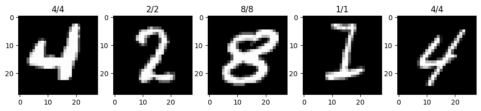
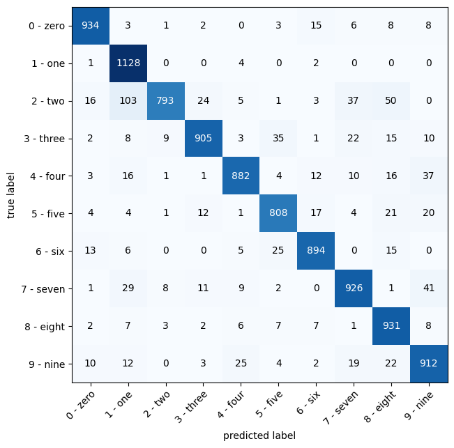
- Plot a confusion matrix comparing your model's predictions to the truth labels.
y_preds_numbers = []
model_e = model_e.to(device)
model_e.eval()
with torch.inference_mode():
    for X, y in tqdm(test_dataloader, desc="Making predictions..."):
        # Send the data and targets to target device
        X, y = X.to(device), y.to(device)

        # Do the forward pass
        y_logit = model_e(X)

        # Turn predictions from logits -> prediction probabilities -> prediction labels
        y_pred = torch.softmax(y_logit.squeeze(), dim=0).argmax(dim=1)

        # Put predictions on cpu for evaluations
        y_preds_numbers.append(y_pred.cpu())

# Concatenate list of predictions into tensor
print(y_preds_numbers[0].shape)
y_pred_tensor_numbers = torch.cat(y_preds_numbers)
print(y_pred_tensor_numbers.shape)
y_pred_tensor_numbers[:10]{"model_id":"daf25c1feec24b0a8cd7a3b387378a0a","version_major":2,"version_minor":0}torch.Size([32])
torch.Size([10000])
tensor([7, 2, 1, 0, 4, 1, 8, 8, 8, 9])from torchmetrics import ConfusionMatrix
from mlxtend.plotting import plot_confusion_matrix
# 2. Setup confusion instance and compare predictions to targets
confmat = ConfusionMatrix(task='multiclass', num_classes=len(mnist_test.classes))
confmat_tensor = confmat(preds=y_pred_tensor_numbers,
target=mnist_test.targets)
# 3. Plot the confusion matrix
fig, ax = plot_confusion_matrix(
conf_mat=confmat_tensor.numpy(), # matplotlib likes working with numpy
class_names=mnist_test.classes,
figsize=(10, 7)
)
- Create a random tensor of shape [1, 3, 64, 64] and pass it through a nn.Conv2d() layer with various hyperparameter settings (these can be any settings you choose), what do you notice if the kernel_size parameter goes up and down?
with torch.inference_mode():
    random_tensor = torch.rand(size=(1, 3, 64, 64))
    conv_layer = nn.Conv2d(in_channels=3,
                      out_channels=2,
                      kernel_size=64,
                      padding=0,
                      stride=1)

result = conv_layer(random_tensor)
result.shape, result
(torch.Size([1, 2, 1, 1]),
tensor([[[[-0.3473]],
[[ 0.2667]]]]))
Начал четвертую часть