Понедельник, 17 Июня 2024

Прошел первую часть курса по пайторчу. Вот ноутбук

what_were_covering = {
    1: "data (prepare and load)",
    2: "build model",
    3: "fitting the model to data (training)",
    4: "making predictions and evaluating a model (inference)",
    5: "saving and loading a model",
    6: "putting it all together"
}

import torch
from torch import nn
import matplotlib.pyplot as plt

torch.__version__

'2.1.2+cpu'

Data (prepare and loading)

excel spreadsheet
images
videos
audio
DNA
text

Machine learning is a game of 2 parts:

Get data into a numerical representation
Build a model to learn patterns in that numerical representation

To showcase this, let's create some known data using linear regression formula

Y = a + bX

We'll use a linear regression formula to make a straight line with known parameters

# Create *known* parameters

weight = 0.7 # b
bias = 0.3   # a

# Create
start = 0
end = 1
step = 0.02

X = torch.arange(start, end, step).unsqueeze(dim=1)
y = weight * X + bias

[f"{a}, {b}" for a, b in zip(X[:10], y[:10])]

['tensor([0.]), tensor([0.3000])',
 'tensor([0.0200]), tensor([0.3140])',
 'tensor([0.0400]), tensor([0.3280])',
 'tensor([0.0600]), tensor([0.3420])',
 'tensor([0.0800]), tensor([0.3560])',
 'tensor([0.1000]), tensor([0.3700])',
 'tensor([0.1200]), tensor([0.3840])',
 'tensor([0.1400]), tensor([0.3980])',
 'tensor([0.1600]), tensor([0.4120])',
 'tensor([0.1800]), tensor([0.4260])']

len(X), len(y)

(50, 50)

Splitting data into training and test sets

(one of the most important concepts in machine learning in general)

three datasets

training set
validation set
test set

Let's create training and test set

# create train/test split
train_split = int(0.8 * len(X))
X_train, y_train = X[:train_split], y[:train_split]
X_test, y_test = X[train_split:], y[train_split:]

len(X_train), len(y_train), len(X_test), len(y_test)

(40, 40, 10, 10)

How might we better visualize our data?

There is where the data explorer's motto comes in!

"Visualize, visualize, visualize!"

def plot_predictions(train_data=X_train,
                    train_labels=y_train,
                    test_data=X_test,
                    test_labels=y_test,
                    predictions=None):
    """
    Plots training data, test data and compares predictions.
    """
    plt.figure(figsize=(10, 7))
    
    # Plot training data in blue
    plt.scatter(train_data, train_labels, c="b", label="Training data")
    
    # Plot testing data in green
    plt.scatter(test_data, test_labels, c="g", label="Testing data")
    
    # Are there predictions
    if predictions is not None:
        plt.scatter(test_data, predictions, c="r", s=4, label="Predictions")
        
    plt.legend(prop={"size": 14})

plot_predictions()

2. Build model

Our first Pytorch model

This is very excited... let's do it

What our model does:

Start with random values (weight & bias)
Look at training data and adjust the random values to better represent(or to get closer to) the ideal values (the weight & bias values we used to create data)

How does it do so?

Gradient descent
Backpropogation

from torch import nn
# Create linear regression model class

class LinearRegressionModel(nn.Module):
    def __init__(self):
        super().__init__()
        self.weight = nn.Parameter(torch.randn(1,
                                               requires_grad=True,
                                               dtype=torch.float))
        self.bias = nn.Parameter(torch.randn(1, 
                                             requires_grad=True,
                                             dtype=torch.float))
        # forward method to define the computation in the model
    def forward(self, x: torch.Tensor) -> torch.Tensor:
        return self.weight * x + self.bias

Pytorch model building essentials

torch.nn - contains all of the buildings for computational graphs (a neural net can be considered as a computational graph)
torch.nn.Parameter - what parameters should our model try and learn, often a PyTorch layer from torch.nn will set these for us
torch.nn.Module - the base class for all neural network modules, if you subclass it, you should overwrite forward()
torch.optim - this is where the optimizers in Pytorch live, they will help with gradient descent.
def forward() - all nn.Module subclasses require you to overwrite forward(), this method defines what happens in the forward computation

pytorch cheat sheet https://pytorch.org/tutorials/beginner/ptcheat.html

Checking the contents of our PyTorch model

Now we've created a model. Let's check what's inside.

So we can check our model parameters or what's inside our model using .parameters()

torch.manual_seed(42)

model_0 = LinearRegressionModel()

list(model_0.parameters())

[Parameter containing:
 tensor([0.3367], requires_grad=True),
 Parameter containing:
 tensor([0.1288], requires_grad=True)]

model_0.state_dict()

OrderedDict([('weight', tensor([0.3367])), ('bias', tensor([0.1288]))])

weight, bias

(0.7, 0.3)

Making prediction using `torch.inference_mode()`

To check our model's predictive power, let's see how well it predicts y_test based on X_test

When we pass data through our model, it's going to run it through forward() method

with torch.inference_mode():
    y_preds = model_0(X_test)
    
y_preds

tensor([[0.3982],
        [0.4049],
        [0.4116],
        [0.4184],
        [0.4251],
        [0.4318],
        [0.4386],
        [0.4453],
        [0.4520],
        [0.4588]])

y_test

tensor([[0.8600],
        [0.8740],
        [0.8880],
        [0.9020],
        [0.9160],
        [0.9300],
        [0.9440],
        [0.9580],
        [0.9720],
        [0.9860]])

plot_predictions(predictions=y_preds)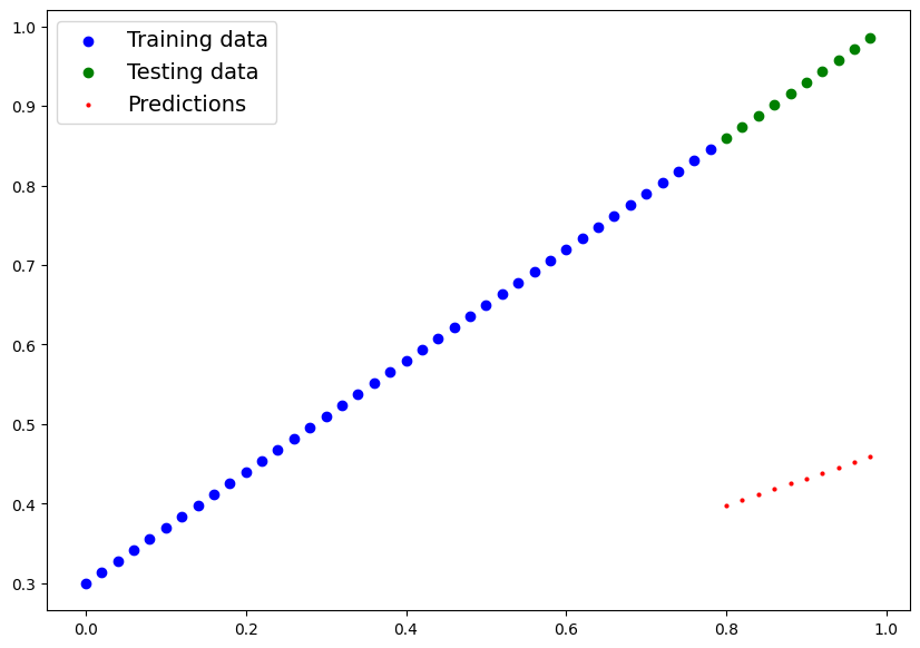

3. Train model

The whole idea of training is for a model to move from some unknown parameters (these may be random) to some known parameters.

Or in other words from a poor representation of the data to a better representation of the data.

One way to measure how poor or how wrong your models predictions are is to use a loss function.

Note: Loss function may also be called cost function or criterion in different areas. For our case, we're going to refer to it as a loss function.

Things we need to train:

Loss function: A function to measure how wrong your model's predictions are to the ideal outputs, lower is better.
Optimizer: Takes into account the loss of a model and adjusts the model's parameters (e.g. weight&bias) to improve the loss function.

And specifically for PyTorch, we need:

A training loop
A testing loop

model_0.state_dict()

OrderedDict([('weight', tensor([0.3367])), ('bias', tensor([0.1288]))])

# Setup a loss function

loss_fn = nn.L1Loss()

# Setup an optimizer
optimizer = torch.optim.SGD(
    params = model_0.parameters(),
    lr = 0.01)

loss_fn, optimizer

(L1Loss(),
 SGD (
 Parameter Group 0
     dampening: 0
     differentiable: False
     foreach: None
     lr: 0.01
     maximize: False
     momentum: 0
     nesterov: False
     weight_decay: 0
 ))

Building a training loop (and testing loop) in Pytorch

A couple of things we need in training loop:
Loop through the data and do...

Forward pass (this involves data moving through our model's forward function) to make predictions on data - also called forward propogation
Calculate the loss (compare forward pass predicitons to ground truth labels)
Optimizer zero grad
Loss backward - move backwards through the network to calculate the gradients of each of the parameters of our model with respect to the loss (back propogarion)
Optimizer step - use the optimizer to adjust our model's parameters to try and improve the loss(gradient descent)

torch.manual_seed(42)
# An epoch is one loop through the data
epochs = 200

# Track different values
epoch_count = []
loss_values = []
test_loss_values = []

### Training
# Loop through the data
for epoch in range(epochs):
    # Set the model to training mode
    model_0.train() # train mode sets all parameters the require gradients to require gradients
    
    # 1. Forward pass
    y_preds = model_0(X_train)
    
    # 2. Calculate loss
    loss = loss_fn(y_preds, y_train)
    #print(f"Loss: {loss}")
    
    # 3. Optimizer zero grad
    optimizer.zero_grad()
    
    # 4. Perform backpropogation
    loss.backward()
    
    # 5. Step the optimizer (perform gradient descent)
    optimizer.step() # by default the optimizer changes will accumulate through the loop so... we have to zero them in step 3 for the next iteration of the loop
    
    
    ### Testing
    model_0.eval() ## turns off gradient tracking

    with torch.inference_mode():
        # 1. Do forward pass
        test_pred = model_0(X_test)
        
        # 2. calculate the loss
        test_loss = loss_fn(test_pred, y_test)
        
    # Print what's happening
    if epoch % 10 == 0:   
        epoch_count.append(epoch)
        loss_values.append(loss)
        test_loss_values.append(test_loss)
        print(f"Epoch: {epoch} | Loss: {loss}: Test loss: {test_loss}")

Epoch: 0 | Loss: 0.31288138031959534: Test loss: 0.48106518387794495
Epoch: 10 | Loss: 0.1976713240146637: Test loss: 0.3463551998138428
Epoch: 20 | Loss: 0.08908725529909134: Test loss: 0.21729660034179688
Epoch: 30 | Loss: 0.053148526698350906: Test loss: 0.14464017748832703
Epoch: 40 | Loss: 0.04543796554207802: Test loss: 0.11360953003168106
Epoch: 50 | Loss: 0.04167863354086876: Test loss: 0.09919948130846024
Epoch: 60 | Loss: 0.03818932920694351: Test loss: 0.08886633068323135
Epoch: 70 | Loss: 0.03476089984178543: Test loss: 0.0805937647819519
Epoch: 80 | Loss: 0.03132382780313492: Test loss: 0.07232122868299484
Epoch: 90 | Loss: 0.02788739837706089: Test loss: 0.06473556160926819
Epoch: 100 | Loss: 0.024458957836031914: Test loss: 0.05646304413676262
Epoch: 110 | Loss: 0.021020207554101944: Test loss: 0.04819049686193466
Epoch: 120 | Loss: 0.01758546568453312: Test loss: 0.04060482233762741
Epoch: 130 | Loss: 0.014155393466353416: Test loss: 0.03233227878808975
Epoch: 140 | Loss: 0.010716589167714119: Test loss: 0.024059748277068138
Epoch: 150 | Loss: 0.0072835334576666355: Test loss: 0.016474086791276932
Epoch: 160 | Loss: 0.0038517764769494534: Test loss: 0.008201557211577892
Epoch: 170 | Loss: 0.008932482451200485: Test loss: 0.005023092031478882
Epoch: 180 | Loss: 0.008932482451200485: Test loss: 0.005023092031478882
Epoch: 190 | Loss: 0.008932482451200485: Test loss: 0.005023092031478882

model_0.state_dict()

OrderedDict([('weight', tensor([0.6990])), ('bias', tensor([0.3093]))])

y_preds = model_0(X_test)
plot_predictions(predictions=y_preds.detach().numpy())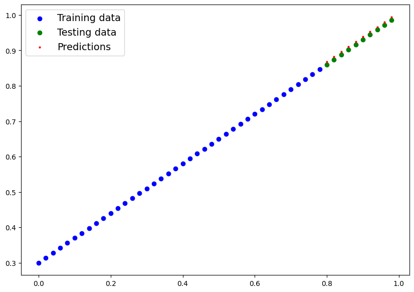

# Plot the loss curves
with torch.no_grad():
    plt.plot(epoch_count, loss_values, label="Train loss")
    plt.plot(epoch_count, test_loss_values, label="Test loss")
    plt.title("Training and test loss curves")
    plt.ylabel("Loss")
    plt.xlabel("Epochs")
    plt.legend()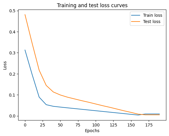

Saving a model in PyTorch

There are three main methods you should know about for saving and loading models in pytorch

torch.save() - allow you to save pytorch object in pickle format
torch.load() - allow you to load saved pytorch object
torch.nn.Module.load_state_dict() - this allows to load a model's saved state dictionary

model_0.state_dict()

OrderedDict([('weight', tensor([0.6990])), ('bias', tensor([0.3093]))])

# Saving our PyTorch model
from pathlib import Path

# 1. Create models directory
MODEL_PATH = Path("models")
MODEL_PATH.mkdir(parents=True, exist_ok=True)

# 2. Create model save path
MODEL_NAME = "01_pytorch_workflow_model_0.pth"
MODEL_SAVE_PATH = MODEL_PATH / MODEL_NAME

MODEL_SAVE_PATH

PosixPath('models/01_pytorch_workflow_model_0.pth')

# 3. Save the model's state dict
torch.save(obj=model_0.state_dict(), f=MODEL_SAVE_PATH)

! ls -l models

/opt/conda/lib/python3.10/pty.py:89: RuntimeWarning: os.fork() was called. os.fork() is incompatible with multithreaded code, and JAX is multithreaded, so this will likely lead to a deadlock.
  pid, fd = os.forkpty()

total 4
-rw-r--r-- 1 root root 1680 Jun 17 13:24 01_pytorch_workflow_model_0.pth

Loading a PyTorch model

Since we saved our model's state_dict() rather the entire model, we'll create a new instance of our model class and load the saved state_dict into that

# To load in a saved state_dict we have to instatiate a new instance of our model class
loaded_model_0 = LinearRegressionModel()

loaded_model_0.state_dict()

OrderedDict([('weight', tensor([0.3367])), ('bias', tensor([0.1288]))])

# Load the saved state dict of model_0
loaded_model_0.load_state_dict(torch.load(f=MODEL_SAVE_PATH))

<All keys matched successfully>

loaded_model_0.state_dict()

OrderedDict([('weight', tensor([0.6990])), ('bias', tensor([0.3093]))])

loaded_model_0.eval()
with torch.inference_mode():
    loaded_model_preds = loaded_model_0(X_test)
    
loaded_model_preds

tensor([[0.8685],
        [0.8825],
        [0.8965],
        [0.9105],
        [0.9245],
        [0.9384],
        [0.9524],
        [0.9664],
        [0.9804],
        [0.9944]])

plot_predictions(predictions=loaded_model_preds)

y_preds, loaded_model_preds

(tensor([[0.8685],
         [0.8825],
         [0.8965],
         [0.9105],
         [0.9245],
         [0.9384],
         [0.9524],
         [0.9664],
         [0.9804],
         [0.9944]], grad_fn=<AddBackward0>),
 tensor([[0.8685],
         [0.8825],
         [0.8965],
         [0.9105],
         [0.9245],
         [0.9384],
         [0.9524],
         [0.9664],
         [0.9804],
         [0.9944]]))

y_preds == loaded_model_preds

tensor([[True],
        [True],
        [True],
        [True],
        [True],
        [True],
        [True],
        [True],
        [True],
        [True]])

6. Putting it all together

Let's go back through the steps above and see it all in one place

# Import Pytorch and matplotlib
import torch
from torch import nn
import matplotlib.pyplot as plt

# Check pytorch version
torch.__version__

'2.1.2+cpu'

# Create device agnostic code
device = "cuda" if torch.cuda.is_available() else "cpu"
device

'cpu'

6.1 Data

# Create some data using linear regression formula
weight = 0.7
bias = 0.3

# Create range values
start = 0
end = 1
step = 0.02

# Create X and y (fratures and labels)
X = torch.arange(start, end, step).unsqueeze(dim=1)
X = weight * X + bias

X[:10], y[:10]

(tensor([[0.3000],
         [0.3140],
         [0.3280],
         [0.3420],
         [0.3560],
         [0.3700],
         [0.3840],
         [0.3980],
         [0.4120],
         [0.4260]]),
 tensor([[0.3000],
         [0.3140],
         [0.3280],
         [0.3420],
         [0.3560],
         [0.3700],
         [0.3840],
         [0.3980],
         [0.4120],
         [0.4260]]))

# Split data
train_split = int(0.8 * len(X))
X_train, y_train = X[:train_split], y[:train_split]
X_test, y_test = X[train_split:], y[train_split:]
len(X_train), len(y_train), len(X_test), len(y_test)

(40, 40, 10, 10)

plot_predictions(X_train, y_train, X_test, y_test)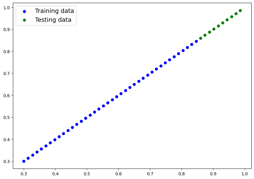

6.2 Building PyTorch linear model

# Create a linear model by subclassing nn.Module
class LinearRegressionModelV2(nn.Module):
    def __init__(self):
        super().__init__()
        # use nn.Linear() for creating the model parameters
        # also called linear transform, probing layer, fully connected layer, dense layer
        self.linear_layer = nn.Linear(
            in_features=1,
            out_features=1
        )
        
    def forward(self, x: torch.Tensor) -> torch.Tensor:
        return self.linear_layer(x)

torch.manual_seed(42)
model_1 = LinearRegressionModelV2()
model_1, model_1.state_dict()

(LinearRegressionModelV2(
   (linear_layer): Linear(in_features=1, out_features=1, bias=True)
 ),
 OrderedDict([('linear_layer.weight', tensor([[0.7645]])),
              ('linear_layer.bias', tensor([0.8300]))]))

# check the model current device
next(model_1.parameters()).device

device(type='cpu')

# Set the model to use the target device
model_1.to(device)
next(model_1.parameters()).device

device(type='cpu')

6.3 Training

For training we need:

Loss function
Optimizer
Training loop
Testing loop

loss_fn = nn.L1Loss()
optimizer = torch.optim.SGD(params=model_1.parameters(), lr=0.01)

# Put data on target device
X_train = X_train.to(device)
y_train = y_train.to(device)
X_test = X_test.to(device)
y_test = y_test.to(device)

torch.manual_seed(42)

epochs = 2000

for epoch in range(epochs):
    # Training
    model_1.train()
    
    y_pred = model_1(X_train)
    
    loss = loss_fn(y_pred, y_train)
    
    optimizer.zero_grad()
    
    loss.backward()
    
    optimizer.step()
    
    # Testing
    model_1.eval()
    
    with torch.inference_mode():
        test_pred = model_1(X_test)
        
        test_loss = loss_fn(test_pred, y_test)
        
    if epoch % 10 == 0:
        print(f"Epoch: {epoch} | Loss {loss} | Test Loss {test_loss}")

Epoch: 0 | Loss 0.6950885057449341 | Test Loss 0.5973882079124451
Epoch: 10 | Loss 0.562255859375 | Test Loss 0.4445006251335144
Epoch: 20 | Loss 0.4294232428073883 | Test Loss 0.2916131019592285
Epoch: 30 | Loss 0.29659053683280945 | Test Loss 0.13872551918029785
Epoch: 40 | Loss 0.16375789046287537 | Test Loss 0.019494276493787766
Epoch: 50 | Loss 0.08495063334703445 | Test Loss 0.11849091202020645
Epoch: 60 | Loss 0.07428932189941406 | Test Loss 0.15105655789375305
Epoch: 70 | Loss 0.07158394902944565 | Test Loss 0.16059081256389618
Epoch: 80 | Loss 0.06992298364639282 | Test Loss 0.1630866825580597
Epoch: 90 | Loss 0.06844298541545868 | Test Loss 0.16016355156898499
Epoch: 100 | Loss 0.06697963178157806 | Test Loss 0.1564663052558899
Epoch: 110 | Loss 0.06551346182823181 | Test Loss 0.15276901423931122
Epoch: 120 | Loss 0.0640547126531601 | Test Loss 0.1498459130525589
Epoch: 130 | Loss 0.06258906424045563 | Test Loss 0.1461486518383026
Epoch: 140 | Loss 0.06112288683652878 | Test Loss 0.14245137572288513
Epoch: 150 | Loss 0.05966467410326004 | Test Loss 0.1395282745361328
Epoch: 160 | Loss 0.05819849297404289 | Test Loss 0.13583102822303772
Epoch: 170 | Loss 0.05673231557011604 | Test Loss 0.13213381171226501
Epoch: 180 | Loss 0.055274106562137604 | Test Loss 0.1292107254266739
Epoch: 190 | Loss 0.053807925432920456 | Test Loss 0.12551352381706238
Epoch: 200 | Loss 0.052344001829624176 | Test Loss 0.12259042263031006
Epoch: 210 | Loss 0.05088352411985397 | Test Loss 0.11889319121837616
Epoch: 220 | Loss 0.049417342990636826 | Test Loss 0.11519596725702286
Epoch: 230 | Loss 0.0479557067155838 | Test Loss 0.11227288097143173
Epoch: 240 | Loss 0.04649295285344124 | Test Loss 0.10857568681240082
Epoch: 250 | Loss 0.04502677917480469 | Test Loss 0.10487842559814453
Epoch: 260 | Loss 0.043567411601543427 | Test Loss 0.1019553691148758
Epoch: 270 | Loss 0.0421023815870285 | Test Loss 0.0982581377029419
Epoch: 280 | Loss 0.040636204183101654 | Test Loss 0.09456091374158859
Epoch: 290 | Loss 0.03917798399925232 | Test Loss 0.09163784235715866
Epoch: 300 | Loss 0.03771181032061577 | Test Loss 0.08794058859348297
Epoch: 310 | Loss 0.03624562546610832 | Test Loss 0.08424339443445206
Epoch: 320 | Loss 0.03478741645812988 | Test Loss 0.08132028579711914
Epoch: 330 | Loss 0.03332122415304184 | Test Loss 0.07762306183576584
Epoch: 340 | Loss 0.03185669332742691 | Test Loss 0.0747000128030777
Epoch: 350 | Loss 0.030396845191717148 | Test Loss 0.07100275158882141
Epoch: 360 | Loss 0.0289306640625 | Test Loss 0.0673055499792099
Epoch: 370 | Loss 0.027468383312225342 | Test Loss 0.06438252329826355
Epoch: 380 | Loss 0.026006245985627174 | Test Loss 0.06068538501858711
Epoch: 390 | Loss 0.02454007789492607 | Test Loss 0.056988220661878586
Epoch: 400 | Loss 0.023080071434378624 | Test Loss 0.054065216332674026
Epoch: 410 | Loss 0.021615678444504738 | Test Loss 0.05036801099777222
Epoch: 420 | Loss 0.020149504765868187 | Test Loss 0.04667087644338608
Epoch: 430 | Loss 0.018691271543502808 | Test Loss 0.043747853487730026
Epoch: 440 | Loss 0.017225103452801704 | Test Loss 0.04005064442753792
Epoch: 450 | Loss 0.015758907422423363 | Test Loss 0.036353498697280884
Epoch: 460 | Loss 0.014300691895186901 | Test Loss 0.03343048691749573
Epoch: 470 | Loss 0.012834521941840649 | Test Loss 0.029733281582593918
Epoch: 480 | Loss 0.011369312182068825 | Test Loss 0.02681024745106697
Epoch: 490 | Loss 0.009910115040838718 | Test Loss 0.02311309054493904
Epoch: 500 | Loss 0.008443924598395824 | Test Loss 0.01941591501235962
Epoch: 510 | Loss 0.006981014274060726 | Test Loss 0.01649288460612297
Epoch: 520 | Loss 0.005519521422684193 | Test Loss 0.012795686721801758
Epoch: 530 | Loss 0.004054142627865076 | Test Loss 0.00910497922450304
Epoch: 540 | Loss 0.002660332713276148 | Test Loss 0.0070143043994903564
Epoch: 550 | Loss 0.0063979425467550755 | Test Loss 0.013234853744506836
Epoch: 560 | Loss 0.0063979425467550755 | Test Loss 0.013234853744506836
Epoch: 570 | Loss 0.0063979425467550755 | Test Loss 0.013234853744506836
Epoch: 580 | Loss 0.0063979425467550755 | Test Loss 0.013234853744506836
Epoch: 590 | Loss 0.0063979425467550755 | Test Loss 0.013234853744506836
Epoch: 600 | Loss 0.0063979425467550755 | Test Loss 0.013234853744506836
Epoch: 610 | Loss 0.0063979425467550755 | Test Loss 0.013234853744506836
Epoch: 620 | Loss 0.0063979425467550755 | Test Loss 0.013234853744506836
Epoch: 630 | Loss 0.0063979425467550755 | Test Loss 0.013234853744506836
Epoch: 640 | Loss 0.0063979425467550755 | Test Loss 0.013234853744506836
Epoch: 650 | Loss 0.0063979425467550755 | Test Loss 0.013234853744506836
Epoch: 660 | Loss 0.0063979425467550755 | Test Loss 0.013234853744506836
Epoch: 670 | Loss 0.0063979425467550755 | Test Loss 0.013234853744506836
Epoch: 680 | Loss 0.0063979425467550755 | Test Loss 0.013234853744506836
Epoch: 690 | Loss 0.0063979425467550755 | Test Loss 0.013234853744506836
Epoch: 700 | Loss 0.0063979425467550755 | Test Loss 0.013234853744506836
Epoch: 710 | Loss 0.0063979425467550755 | Test Loss 0.013234853744506836
Epoch: 720 | Loss 0.0063979425467550755 | Test Loss 0.013234853744506836
Epoch: 730 | Loss 0.0063979425467550755 | Test Loss 0.013234853744506836
Epoch: 740 | Loss 0.0063979425467550755 | Test Loss 0.013234853744506836
Epoch: 750 | Loss 0.0063979425467550755 | Test Loss 0.013234853744506836
Epoch: 760 | Loss 0.0063979425467550755 | Test Loss 0.013234853744506836
Epoch: 770 | Loss 0.0063979425467550755 | Test Loss 0.013234853744506836
Epoch: 780 | Loss 0.0063979425467550755 | Test Loss 0.013234853744506836
Epoch: 790 | Loss 0.0063979425467550755 | Test Loss 0.013234853744506836
Epoch: 800 | Loss 0.0063979425467550755 | Test Loss 0.013234853744506836
Epoch: 810 | Loss 0.0063979425467550755 | Test Loss 0.013234853744506836
Epoch: 820 | Loss 0.0063979425467550755 | Test Loss 0.013234853744506836
Epoch: 830 | Loss 0.0063979425467550755 | Test Loss 0.013234853744506836
Epoch: 840 | Loss 0.0063979425467550755 | Test Loss 0.013234853744506836
Epoch: 850 | Loss 0.0063979425467550755 | Test Loss 0.013234853744506836
Epoch: 860 | Loss 0.0063979425467550755 | Test Loss 0.013234853744506836
Epoch: 870 | Loss 0.0063979425467550755 | Test Loss 0.013234853744506836
Epoch: 880 | Loss 0.0063979425467550755 | Test Loss 0.013234853744506836
Epoch: 890 | Loss 0.0063979425467550755 | Test Loss 0.013234853744506836
Epoch: 900 | Loss 0.0063979425467550755 | Test Loss 0.013234853744506836
Epoch: 910 | Loss 0.0063979425467550755 | Test Loss 0.013234853744506836
Epoch: 920 | Loss 0.0063979425467550755 | Test Loss 0.013234853744506836
Epoch: 930 | Loss 0.0063979425467550755 | Test Loss 0.013234853744506836
Epoch: 940 | Loss 0.0063979425467550755 | Test Loss 0.013234853744506836
Epoch: 950 | Loss 0.0063979425467550755 | Test Loss 0.013234853744506836
Epoch: 960 | Loss 0.0063979425467550755 | Test Loss 0.013234853744506836
Epoch: 970 | Loss 0.0063979425467550755 | Test Loss 0.013234853744506836
Epoch: 980 | Loss 0.0063979425467550755 | Test Loss 0.013234853744506836
Epoch: 990 | Loss 0.0063979425467550755 | Test Loss 0.013234853744506836
Epoch: 1000 | Loss 0.0063979425467550755 | Test Loss 0.013234853744506836
Epoch: 1010 | Loss 0.0063979425467550755 | Test Loss 0.013234853744506836
Epoch: 1020 | Loss 0.0063979425467550755 | Test Loss 0.013234853744506836
Epoch: 1030 | Loss 0.0063979425467550755 | Test Loss 0.013234853744506836
Epoch: 1040 | Loss 0.0063979425467550755 | Test Loss 0.013234853744506836
Epoch: 1050 | Loss 0.0063979425467550755 | Test Loss 0.013234853744506836
Epoch: 1060 | Loss 0.0063979425467550755 | Test Loss 0.013234853744506836
Epoch: 1070 | Loss 0.0063979425467550755 | Test Loss 0.013234853744506836
Epoch: 1080 | Loss 0.0063979425467550755 | Test Loss 0.013234853744506836
Epoch: 1090 | Loss 0.0063979425467550755 | Test Loss 0.013234853744506836
Epoch: 1100 | Loss 0.0063979425467550755 | Test Loss 0.013234853744506836
Epoch: 1110 | Loss 0.0063979425467550755 | Test Loss 0.013234853744506836
Epoch: 1120 | Loss 0.0063979425467550755 | Test Loss 0.013234853744506836
Epoch: 1130 | Loss 0.0063979425467550755 | Test Loss 0.013234853744506836
Epoch: 1140 | Loss 0.0063979425467550755 | Test Loss 0.013234853744506836
Epoch: 1150 | Loss 0.0063979425467550755 | Test Loss 0.013234853744506836
Epoch: 1160 | Loss 0.0063979425467550755 | Test Loss 0.013234853744506836
Epoch: 1170 | Loss 0.0063979425467550755 | Test Loss 0.013234853744506836
Epoch: 1180 | Loss 0.0063979425467550755 | Test Loss 0.013234853744506836
Epoch: 1190 | Loss 0.0063979425467550755 | Test Loss 0.013234853744506836
Epoch: 1200 | Loss 0.0063979425467550755 | Test Loss 0.013234853744506836
Epoch: 1210 | Loss 0.0063979425467550755 | Test Loss 0.013234853744506836
Epoch: 1220 | Loss 0.0063979425467550755 | Test Loss 0.013234853744506836
Epoch: 1230 | Loss 0.0063979425467550755 | Test Loss 0.013234853744506836
Epoch: 1240 | Loss 0.0063979425467550755 | Test Loss 0.013234853744506836
Epoch: 1250 | Loss 0.0063979425467550755 | Test Loss 0.013234853744506836
Epoch: 1260 | Loss 0.0063979425467550755 | Test Loss 0.013234853744506836
Epoch: 1270 | Loss 0.0063979425467550755 | Test Loss 0.013234853744506836
Epoch: 1280 | Loss 0.0063979425467550755 | Test Loss 0.013234853744506836
Epoch: 1290 | Loss 0.0063979425467550755 | Test Loss 0.013234853744506836
Epoch: 1300 | Loss 0.0063979425467550755 | Test Loss 0.013234853744506836
Epoch: 1310 | Loss 0.0063979425467550755 | Test Loss 0.013234853744506836
Epoch: 1320 | Loss 0.0063979425467550755 | Test Loss 0.013234853744506836
Epoch: 1330 | Loss 0.0063979425467550755 | Test Loss 0.013234853744506836
Epoch: 1340 | Loss 0.0063979425467550755 | Test Loss 0.013234853744506836
Epoch: 1350 | Loss 0.0063979425467550755 | Test Loss 0.013234853744506836
Epoch: 1360 | Loss 0.0063979425467550755 | Test Loss 0.013234853744506836
Epoch: 1370 | Loss 0.0063979425467550755 | Test Loss 0.013234853744506836
Epoch: 1380 | Loss 0.0063979425467550755 | Test Loss 0.013234853744506836
Epoch: 1390 | Loss 0.0063979425467550755 | Test Loss 0.013234853744506836
Epoch: 1400 | Loss 0.0063979425467550755 | Test Loss 0.013234853744506836
Epoch: 1410 | Loss 0.0063979425467550755 | Test Loss 0.013234853744506836
Epoch: 1420 | Loss 0.0063979425467550755 | Test Loss 0.013234853744506836
Epoch: 1430 | Loss 0.0063979425467550755 | Test Loss 0.013234853744506836
Epoch: 1440 | Loss 0.0063979425467550755 | Test Loss 0.013234853744506836
Epoch: 1450 | Loss 0.0063979425467550755 | Test Loss 0.013234853744506836
Epoch: 1460 | Loss 0.0063979425467550755 | Test Loss 0.013234853744506836
Epoch: 1470 | Loss 0.0063979425467550755 | Test Loss 0.013234853744506836
Epoch: 1480 | Loss 0.0063979425467550755 | Test Loss 0.013234853744506836
Epoch: 1490 | Loss 0.0063979425467550755 | Test Loss 0.013234853744506836
Epoch: 1500 | Loss 0.0063979425467550755 | Test Loss 0.013234853744506836
Epoch: 1510 | Loss 0.0063979425467550755 | Test Loss 0.013234853744506836
Epoch: 1520 | Loss 0.0063979425467550755 | Test Loss 0.013234853744506836
Epoch: 1530 | Loss 0.0063979425467550755 | Test Loss 0.013234853744506836
Epoch: 1540 | Loss 0.0063979425467550755 | Test Loss 0.013234853744506836
Epoch: 1550 | Loss 0.0063979425467550755 | Test Loss 0.013234853744506836
Epoch: 1560 | Loss 0.0063979425467550755 | Test Loss 0.013234853744506836
Epoch: 1570 | Loss 0.0063979425467550755 | Test Loss 0.013234853744506836
Epoch: 1580 | Loss 0.0063979425467550755 | Test Loss 0.013234853744506836
Epoch: 1590 | Loss 0.0063979425467550755 | Test Loss 0.013234853744506836
Epoch: 1600 | Loss 0.0063979425467550755 | Test Loss 0.013234853744506836
Epoch: 1610 | Loss 0.0063979425467550755 | Test Loss 0.013234853744506836
Epoch: 1620 | Loss 0.0063979425467550755 | Test Loss 0.013234853744506836
Epoch: 1630 | Loss 0.0063979425467550755 | Test Loss 0.013234853744506836
Epoch: 1640 | Loss 0.0063979425467550755 | Test Loss 0.013234853744506836
Epoch: 1650 | Loss 0.0063979425467550755 | Test Loss 0.013234853744506836
Epoch: 1660 | Loss 0.0063979425467550755 | Test Loss 0.013234853744506836
Epoch: 1670 | Loss 0.0063979425467550755 | Test Loss 0.013234853744506836
Epoch: 1680 | Loss 0.0063979425467550755 | Test Loss 0.013234853744506836
Epoch: 1690 | Loss 0.0063979425467550755 | Test Loss 0.013234853744506836
Epoch: 1700 | Loss 0.0063979425467550755 | Test Loss 0.013234853744506836
Epoch: 1710 | Loss 0.0063979425467550755 | Test Loss 0.013234853744506836
Epoch: 1720 | Loss 0.0063979425467550755 | Test Loss 0.013234853744506836
Epoch: 1730 | Loss 0.0063979425467550755 | Test Loss 0.013234853744506836
Epoch: 1740 | Loss 0.0063979425467550755 | Test Loss 0.013234853744506836
Epoch: 1750 | Loss 0.0063979425467550755 | Test Loss 0.013234853744506836
Epoch: 1760 | Loss 0.0063979425467550755 | Test Loss 0.013234853744506836
Epoch: 1770 | Loss 0.0063979425467550755 | Test Loss 0.013234853744506836
Epoch: 1780 | Loss 0.0063979425467550755 | Test Loss 0.013234853744506836
Epoch: 1790 | Loss 0.0063979425467550755 | Test Loss 0.013234853744506836
Epoch: 1800 | Loss 0.0063979425467550755 | Test Loss 0.013234853744506836
Epoch: 1810 | Loss 0.0063979425467550755 | Test Loss 0.013234853744506836
Epoch: 1820 | Loss 0.0063979425467550755 | Test Loss 0.013234853744506836
Epoch: 1830 | Loss 0.0063979425467550755 | Test Loss 0.013234853744506836
Epoch: 1840 | Loss 0.0063979425467550755 | Test Loss 0.013234853744506836
Epoch: 1850 | Loss 0.0063979425467550755 | Test Loss 0.013234853744506836
Epoch: 1860 | Loss 0.0063979425467550755 | Test Loss 0.013234853744506836
Epoch: 1870 | Loss 0.0063979425467550755 | Test Loss 0.013234853744506836
Epoch: 1880 | Loss 0.0063979425467550755 | Test Loss 0.013234853744506836
Epoch: 1890 | Loss 0.0063979425467550755 | Test Loss 0.013234853744506836
Epoch: 1900 | Loss 0.0063979425467550755 | Test Loss 0.013234853744506836
Epoch: 1910 | Loss 0.0063979425467550755 | Test Loss 0.013234853744506836
Epoch: 1920 | Loss 0.0063979425467550755 | Test Loss 0.013234853744506836
Epoch: 1930 | Loss 0.0063979425467550755 | Test Loss 0.013234853744506836
Epoch: 1940 | Loss 0.0063979425467550755 | Test Loss 0.013234853744506836
Epoch: 1950 | Loss 0.0063979425467550755 | Test Loss 0.013234853744506836
Epoch: 1960 | Loss 0.0063979425467550755 | Test Loss 0.013234853744506836
Epoch: 1970 | Loss 0.0063979425467550755 | Test Loss 0.013234853744506836
Epoch: 1980 | Loss 0.0063979425467550755 | Test Loss 0.013234853744506836
Epoch: 1990 | Loss 0.0063979425467550755 | Test Loss 0.013234853744506836

model_1.state_dict()

OrderedDict([('linear_layer.weight', tensor([[0.9876]])),
             ('linear_layer.bias', tensor([0.0135]))])

weight, bias

(0.7, 0.3)

model_1.eval()
with torch.inference_mode():
    y_pred = model_1(X_test)
with torch.no_grad():
    plot_predictions(X_train, y_train, X_test, y_test, predictions=y_pred)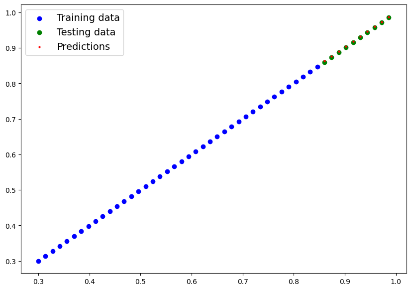

6.5 Saving and loading a trained model

from pathlib import Path
# 1. Create models directory
MODEL_PATH = Path("models")
MODEL_PATH.mkdir(parents=True, exist_ok=True)

# 2. Create model save path
MODEL_NAME = "01_pytorch_workflow_model_1.pth"
MODEL_SAVE_PATH = MODEL_PATH / MODEL_NAME
MODEL_SAVE_PATH

PosixPath('models/01_pytorch_workflow_model_1.pth')

# 3. Save model state dict
torch.save(obj=model_1.state_dict(),f=MODEL_SAVE_PATH)

! ls -l models

total 8
-rw-r--r-- 1 root root 1680 Jun 17 13:24 01_pytorch_workflow_model_0.pth
-rw-r--r-- 1 root root 1744 Jun 17 13:24 01_pytorch_workflow_model_1.pth

# Load a pytorch model

loaded_model_1 = LinearRegressionModelV2()
loaded_model_1.load_state_dict(torch.load(f=MODEL_SAVE_PATH))

<All keys matched successfully>

loaded_model_1.to(device)
loaded_model_1.state_dict()

OrderedDict([('linear_layer.weight', tensor([[0.9876]])),
             ('linear_layer.bias', tensor([0.0135]))])

next(loaded_model_1.parameters()).device

device(type='cpu')

# Evaluate loaded model
loaded_model_1.eval()
with torch.inference_mode():
    loaded_model_1_preds = loaded_model_1(X_test)

with torch.no_grad():
    plot_predictions(X_train, y_train, X_test, y_test, predictions=y_pred)

with torch.no_grad():
    plot_predictions(X_train, y_train, X_test, y_test, predictions=loaded_model_1_preds)

Exercises and extra-curriculum

device = "cuda" if torch.cuda.is_available() else "cpu"

# Create a straight line dataset using the linear regression formula (weight * X + bias).
# Set weight=0.3 and bias=0.9 there should be at least 100 datapoints total.
# Split the data into 80% training, 20% testing.
# Plot the training and testing data so it becomes visual.

weight = 0.3
bias = 0.9

X = torch.arange(0, 1, 0.01).unsqueeze(dim=1)
y = weight * X + bias
X_train, y_train = X[:80], y[:80]
X_test, y_test = X[80:], y[80:]

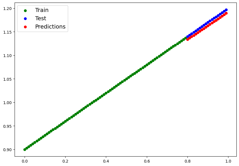
plt.figure(figsize=(10, 7))
plt.scatter(X_train, y_train, c="g", label="Train")
plt.scatter(X_test, y_test, c="b", label="Test")
plt.legend(prop={"size":14})

<matplotlib.legend.Legend at 0x79bb148a63e0>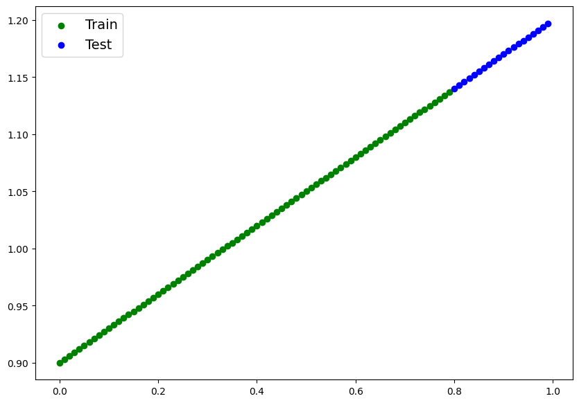

# 2. Build a PyTorch model by subclassing nn.Module.
# Inside should be a randomly initialized nn.Parameter() with requires_grad=True, one for weights and one for bias.
# Implement the forward() method to compute the linear regression function you used to create the dataset in 1.
# Once you've constructed the model, make an instance of it and check its state_dict().
# Note: If you'd like to use nn.Linear() instead of nn.Parameter() you can.

class LinearV3(nn.Module):
    def __init__(self):
        super().__init__()
        self.linear_layer = nn.Linear(in_features=1, out_features=1)
    
    def forward(self, x: torch.Tensor) -> torch.Tensor:
        return self.linear_layer(x)

model_3 = LinearV3()
model_3.state_dict()

OrderedDict([('linear_layer.weight', tensor([[-0.2343]])),
             ('linear_layer.bias', tensor([0.9186]))])

# 3. Create a loss function and optimizer using nn.L1Loss() and torch.optim.SGD(params, lr) respectively.
# Set the learning rate of the optimizer to be 0.01 and the parameters to optimize should be the model parameters from the model you created in 2.
# Write a training loop to perform the appropriate training steps for 300 epochs.
# The training loop should test the model on the test dataset every 20 epochs.

loss_func = nn.L1Loss()
optimizer = torch.optim.SGD(model_3.parameters(), lr=0.01)
epochs = 300

for epoch in range(epochs):
    # Train
    model_3.train()
    
    y_preds_3 = model_3(X_train)
    
    loss = loss_func(y_preds_3, y_train)
    
    optimizer.zero_grad()
    
    loss.backward()
    
    optimizer.step()
    
    # Test
    model_3.eval()
    y_preds_test_3 = model_3(X_test)
    loss_test = loss_func(y_preds_test_3, y_test)
    
    if epoch % 20 == 0:
        print(f"Epoch {epoch} | Loss {loss} | Test loss: {loss_test}")

Epoch 0 | Loss 0.1934860348701477 | Test loss: 0.44704073667526245
Epoch 20 | Loss 0.099742591381073 | Test loss: 0.2774539589881897
Epoch 40 | Loss 0.08286076784133911 | Test loss: 0.20952367782592773
Epoch 60 | Loss 0.07524622231721878 | Test loss: 0.17951278388500214
Epoch 80 | Loss 0.06834527105093002 | Test loss: 0.16077637672424316
Epoch 100 | Loss 0.06149417161941528 | Test loss: 0.1444476842880249
Epoch 120 | Loss 0.05464210361242294 | Test loss: 0.12846292555332184
Epoch 140 | Loss 0.0477910041809082 | Test loss: 0.11213425546884537
Epoch 160 | Loss 0.040939826518297195 | Test loss: 0.09580682963132858
Epoch 180 | Loss 0.03408767282962799 | Test loss: 0.07982330024242401
Epoch 200 | Loss 0.027236470952630043 | Test loss: 0.06349574029445648
Epoch 220 | Loss 0.020384784787893295 | Test loss: 0.04734015464782715
Epoch 240 | Loss 0.013533586636185646 | Test loss: 0.031012600287795067
Epoch 260 | Loss 0.006681408733129501 | Test loss: 0.015028971247375011
Epoch 280 | Loss 0.003223966807126999 | Test loss: 0.006560081150382757

# 4. Make predictions with the trained model on the test data.
# Visualize these predictions against the original training and testing data (note: you may need to make sure the predictions are not on the GPU if you want to use non-CUDA-enabled libraries such as matplotlib to plot).
with torch.inference_mode():
    preds_3 = model_3(X_test)
plt.figure(figsize=(10, 7))
plt.scatter(X_train, y_train, c="g", label="Train")
plt.scatter(X_test, y_test, c="b", label="Test")
plt.scatter(X_test, preds_3, c="r", label="Predictions")
plt.legend(prop={"size":14})

<matplotlib.legend.Legend at 0x79bb148ecd00>

model_3.state_dict()

OrderedDict([('linear_layer.weight', tensor([[0.2925]])),
             ('linear_layer.bias', tensor([0.8997]))])

# Save your trained model's state_dict() to file.
# Create a new instance of your model class you made in 2. and load in the state_dict() you just saved to it.
# Perform predictions on your test data with the loaded model and confirm they match the original model predictions from 4.

from pathlib import Path
SAVE_PATH = "models/model_3.pth"

torch.save(obj=model_3.state_dict(), f=SAVE_PATH)

! ls -l models

total 12
-rw-r--r-- 1 root root 1680 Jun 17 13:24 01_pytorch_workflow_model_0.pth
-rw-r--r-- 1 root root 1744 Jun 17 13:24 01_pytorch_workflow_model_1.pth
-rw-r--r-- 1 root root 1560 Jun 17 13:24 model_3.pth

model_3_loaded = LinearV3()

model_3_loaded.load_state_dict(torch.load(f=SAVE_PATH))

<All keys matched successfully>

with torch.inference_mode():
    preds_3 = model_3_loaded(X_test)
plt.figure(figsize=(10, 7))
plt.scatter(X_train, y_train, c="g", label="Train")
plt.scatter(X_test, y_test, c="b", label="Test")
plt.scatter(X_test, preds_3, c="r", label="Predictions")
plt.legend(prop={"size":14})

<matplotlib.legend.Legend at 0x79bb147a1870>

(Этот же ноутбук на кагле)