Среда, 26 Июня 2024
Прошел вторую часть курса по пайторчу. Вот ноутбук
Neural Network Claasification with PyTorch
Classification is a problem of prediciting whether something is one thing or another (there can be multiple things as the options)
1. Make classification data and get it ready
import sklearn
from sklearn.datasets import make_circles
# Make a 1000 samples
n_samples = 1000
X, y = make_circles(n_samples, noise=0.03, random_state=42)
len(X), len(y)(1000, 1000)X[:5], y[:5](array([[ 0.75424625, 0.23148074],
[-0.75615888, 0.15325888],
[-0.81539193, 0.17328203],
[-0.39373073, 0.69288277],
[ 0.44220765, -0.89672343]]),
array([1, 1, 1, 1, 0]))# Make DataFrame of circle data
import pandas as pd
circles = pd.DataFrame({
"X1": X[:, 0],
"X2": X[:, 1],
"label": y
})
circles.head(10)| X1 | X2 | label | |
|---|---|---|---|
| 0 | 0.754246 | 0.231481 | 1 |
| 1 | -0.756159 | 0.153259 | 1 |
| 2 | -0.815392 | 0.173282 | 1 |
| 3 | -0.393731 | 0.692883 | 1 |
| 4 | 0.442208 | -0.896723 | 0 |
| 5 | -0.479646 | 0.676435 | 1 |
| 6 | -0.013648 | 0.803349 | 1 |
| 7 | 0.771513 | 0.147760 | 1 |
| 8 | -0.169322 | -0.793456 | 1 |
| 9 | -0.121486 | 1.021509 | 0 |
# Visualize, visualize, visualize
import matplotlib.pyplot as plt
plt.scatter(
    x=X[:, 0],
    y=X[:, 1],
    c=y,
    cmap=plt.cm.RdYlBu
)
<matplotlib.collections.PathCollection at 0x7f964a6f4b20>
circles.label.value_counts()label
1 500
0 500
Name: count, dtype: int64Note: The data we're working with is often referred to as a toy dataset, a dataset that is small enough to experiment but still sizeable enough to prectice the fundamentals
1.1 Check input and output shapes
X.shape, y.shape((1000, 2), (1000,))# View the first example of features and labels
X_sample = X[0]
y_sample = y[0]
print(f"Values for one sample of X: {X_sample} and the same for y: {y_sample}")
print(f"Shapes for one sample of X: {X_sample.shape} and the same for y: {y_sample.shape}")Values for one sample of X: [0.75424625 0.23148074] and the same for y: 1
Shapes for one sample of X: (2,) and the same for y: ()
1.2 Turn data into tensors and create train and test split
# Turn data into tensors
import torch

X = torch.from_numpy(X).type(torch.float)
y = torch.from_numpy(y).type(torch.float)X[:5], y[:5](tensor([[ 0.7542, 0.2315],
[-0.7562, 0.1533],
[-0.8154, 0.1733],
[-0.3937, 0.6929],
[ 0.4422, -0.8967]]),
tensor([1., 1., 1., 1., 0.]))# Split data into train and test sets
from sklearn.model_selection import train_test_split
X_train, X_test, y_train, y_test = train_test_split(X, y, test_size=0.2, random_state=42)len(X_train), len(X_test), len(y_train), len(y_test)(800, 200, 800, 200)2. Building a model
Let's build a model to classify our blue and red dots
To do so, we want to:
- Setup device agnostic code so our code will run on an accelerator(GPU) if there is one
- Construct a model (by subclassing nn.Module)
- Define a loss function and optimizer
- Create a training and test loop
# Import Pytorch and nn
import torch
from torch import nn

# Make device agnostic code
device = "cuda" if torch.cuda.is_available() else "cpu"
device'cuda'Now we've setup device agnostic code, let's create a model that:
- Subclasses nn.Module
- Create 2 nn.Linear layers that are capable of handling the shapes of our data
- Define a forward() method
- Instantiate an instance of our model class and send it to the target
device
# 1. Construc a model that subclasses nn.Module

class CircleModelV1(nn.Module):
    def __init__(self):
        super().__init__()
        # 2. Create 2 nn.Linear layers
        # self.layer_1 = nn.Linear(in_features=2, out_features=5) # takes 2 features and upscales to 5 features
        # self.layer_2 = nn.Linear(in_features=5, out_features=1) # takes 5 features from previous layer and outputs a single feature (same shape as y)
        self.two_linear_layers = nn.Sequential(
            nn.Linear(in_features=2, out_features=5),
            nn.Linear(in_features=5, out_features=1)
        )
    # 3. Define forward method
    def forward(self, x):
        return self.two_linear_layers(x) # x-> layer_1 -> layer_2 -> output
# 4. Instantiate an instance of our model class and send it to target device
model_0 = CircleModelV1().to(device)
model_0CircleModelV1(
(two_linear_layers): Sequential(
(0): Linear(in_features=2, out_features=5, bias=True)
(1): Linear(in_features=5, out_features=1, bias=True)
)
)device'cuda'next(model_0.parameters()).devicedevice(type='cuda', index=0)# Let's replicate the model abovee using nn.Sequential()
model_0 = nn.Sequential(
nn.Linear(in_features=2, out_features=5),
nn.Linear(in_features=5, out_features=1)
).to(device)
model_0Sequential(
(0): Linear(in_features=2, out_features=5, bias=True)
(1): Linear(in_features=5, out_features=1, bias=True)
)model_0.state_dict()OrderedDict([('0.weight',
tensor([[ 0.5810, 0.3248],
[ 0.1343, 0.3703],
[ 0.0008, -0.6113],
[-0.6327, 0.6022],
[-0.1916, -0.3258]], device='cuda:0')),
('0.bias',
tensor([-0.5865, 0.6275, 0.3488, 0.0505, -0.2794], device='cuda:0')),
('1.weight',
tensor([[ 0.2281, 0.4445, -0.1389, -0.1189, -0.3437]], device='cuda:0')),
('1.bias', tensor([0.1544], device='cuda:0'))])# Make predictions
with torch.inference_mode():
untrained_preds = model_0(X_test.to(device))
print(f"Length of predictions {len(untrained_preds)}, Shape: {untrained_preds.shape}")
print(f"Length of test samples: {len(X_test)}, Shape: {X_test.shape}")
print(f"First 10 predictions: {torch.round(untrained_preds[:10])}")
print(f"First 10 labels: {y_test[:10]}")Length of predictions 200, Shape: torch.Size([200, 1])
Length of test samples: 200, Shape: torch.Size([200, 2])
First 10 predictions: tensor([[0.],
[1.],
[-0.],
[1.],
[0.],
[0.],
[1.],
[1.],
[-0.],
[1.]], device='cuda:0')
First 10 labels: tensor([1., 0., 1., 0., 1., 1., 0., 0., 1., 0.])
## 2.1 Setup loss function and optimizer
loss_fn = nn.BCEWithLogitsLoss() # BCEWithLogitsLoss has sigmoid activation build in
optimizer = torch.optim.SGD(params=model_0.parameters(), lr=0.1)
# Calculate accuracy - what percentage model predicted right
def accuracy_fn(y_true, y_pred):
correct = torch.eq(y_true, y_pred).sum().item()
acc = (correct/len(y_pred)) * 100
return acc3. Train model
Build training loop
3.1 Going from raw logits -> prediction probabilities -> prediction labels
Our model outputs are going to be raw logits
We can convert logits into prediction probabilities by passing them to some kind of activation function (e.g sigmoid for binary classification and softmax for multiclass classification).
Then we can convert our model's prediction probabilities to prediction labels by either rounding them or taking the argmax()
model_0.eval()
with torch.inference_mode():
    y_logits = model_0(X_test.to(device))[:5]
y_logits
tensor([[ 0.4646],
[ 0.6957],
[-0.0076],
[ 0.5978],
[ 0.2045]], device='cuda:0')y_test[:5]tensor([1., 0., 1., 0., 1.])# Use the sigmoid activation function on our model logits to turn them into prediction probabilities
y_pred_probs = torch.sigmoid(y_logits)
y_pred_probstensor([[0.6141],
[0.6672],
[0.4981],
[0.6452],
[0.5510]], device='cuda:0')# if probability more than or equal 0.5, then label 1, if less 0.5 than 0
y_preds = torch.round(y_pred_probs)
y_preds
# In full (logits -> prediction probobalities -> prediction labels)
y_pred_labels = torch.round(torch.sigmoid(model_0(X_test.to(device)[:5])))
y_pred_labels
# Check for equality
print(torch.eq(y_preds.squeeze(), y_pred_labels.squeeze()))
# Get rid of extra dimension
y_preds.squeeze()tensor([True, True, True, True, True], device='cuda:0')
tensor([1., 1., 0., 1., 1.], device='cuda:0')### Building testing and training loop
torch.manual_seed(42)
torch.cuda.manual_seed(42)
# Set the number of epochs
epochs = 100
# Put data to the target device
X_train, y_train = X_train.to(device), y_train.to(device)
X_test, y_test = X_test.to(device), y_test.to(device)
for epoch in range(epochs):
model_0.train()
# forward pass
y_logits = model_0(X_train).squeeze()
y_pred = torch.round(torch.sigmoid(y_logits))
# calculate the loss and accuracy
loss = loss_fn(y_logits, y_train)
acc = accuracy_fn(y_true=y_train, y_pred=y_pred)
optimizer.zero_grad()
# backpropogation
loss.backward()
# gradient descent
optimizer.step()
### Testing
model_0.eval()
with torch.inference_mode():
test_logits = model_0(X_test).squeeze()
test_pred = torch.round(torch.sigmoid(test_logits))
# calculate test loss and accuracy
test_loss = loss_fn(test_logits, y_test)
test_acc = accuracy_fn(y_true=y_test, y_pred=test_pred)
# print out what happening
if epoch % 10 == 0:
print(f"Epoch: {epoch} | Loss: {loss:.5f}, Acc: {acc:.2f}%| Test loss: {test_loss:.5f}, test acc: {test_acc:.2f}%")Epoch: 0 | Loss: 0.71618, Acc: 55.00%| Test loss: 0.73183, test acc: 50.00%
Epoch: 10 | Loss: 0.70584, Acc: 53.25%| Test loss: 0.72014, test acc: 47.50%
Epoch: 20 | Loss: 0.70166, Acc: 52.50%| Test loss: 0.71459, test acc: 46.50%
Epoch: 30 | Loss: 0.69955, Acc: 51.62%| Test loss: 0.71132, test acc: 47.00%
Epoch: 40 | Loss: 0.69827, Acc: 51.12%| Test loss: 0.70903, test acc: 47.00%
Epoch: 50 | Loss: 0.69736, Acc: 51.00%| Test loss: 0.70728, test acc: 47.50%
Epoch: 60 | Loss: 0.69667, Acc: 51.12%| Test loss: 0.70586, test acc: 47.50%
Epoch: 70 | Loss: 0.69612, Acc: 51.25%| Test loss: 0.70469, test acc: 47.50%
Epoch: 80 | Loss: 0.69568, Acc: 51.38%| Test loss: 0.70369, test acc: 47.50%
Epoch: 90 | Loss: 0.69531, Acc: 51.38%| Test loss: 0.70283, test acc: 47.50%
4. Make predictions and evaluate the model
from metrics it looks like our model isn't learning anything
So to inspect it let's make predictions and make them visual
import requests
from pathlib import Path

# Download helper functions from Learn Pytorch repo

if Path("helper_functions.py").is_file():
    print("already exist")
else:
    request = requests.get("https://raw.githubusercontent.com/mrdbourke/pytorch-deep-learning/main/helper_functions.py")
    with open("helper_functions.py", "wb") as f:
        f.write(request.content)

from helper_functions import plot_predictions, plot_decision_boundary
# Plot decision boundary of the model
plt.figure(figsize=(12, 6))
plt.subplot(1, 2, 1)
plt.title("Train")
plot_decision_boundary(model_0, X_train, y_train)
plt.subplot(1, 2, 2)
plt.title("Test")
plot_decision_boundary(model_0, X_test, y_test)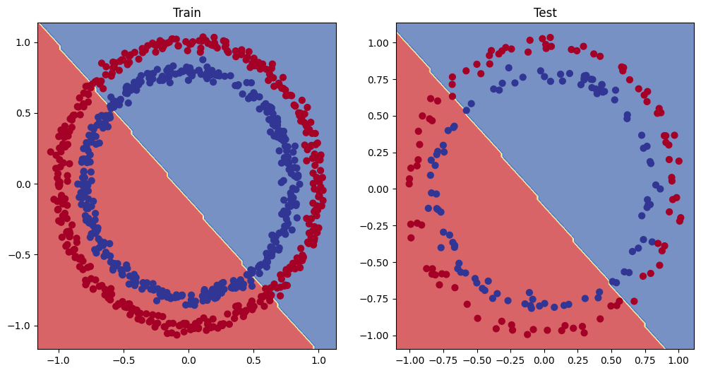
5. Improving a model (from a model perspective)
- Add more layers - give the model more chances to learn about patterns in the data
- Add more hidden units - go from 5 hidden units to 10 hidden units
- Fit for longer
- Changing the activation function
- Change the learning rate
- Change the loss function
These options are all from a model's perspective because they deal directly with the model, rather than the data.
And because these options are all values we (as machine learning engineers and data scientists) can change, they are reffered as hyperparameters
class CircleModelV1(nn.Module):
    def __init__(self):
        super().__init__()
        self.layer_1 = nn.Linear(in_features=2, out_features=10)
        self.layer_2 = nn.Linear(in_features=10, out_features=10)
        self.layer_3 = nn.Linear(in_features=10, out_features=1)

    def forward(self, x):
        return self.layer_3(self.layer_2(self.layer_1(x)))

model_1 = CircleModelV1().to(device)
model_1
CircleModelV1(
(layer_1): Linear(in_features=2, out_features=10, bias=True)
(layer_2): Linear(in_features=10, out_features=10, bias=True)
(layer_3): Linear(in_features=10, out_features=1, bias=True)
)loss_fn = torch.nn.BCEWithLogitsLoss()
optimizer = torch.optim.SGD(params=model_1.parameters(), lr=0.1)### Building testing and training loop
torch.manual_seed(42)
torch.cuda.manual_seed(42)
epochs = 1000
X_train, y_train = X_train.to(device), y_train.to(device)
X_test, y_test = X_test.to(device), y_test.to(device)
for epoch in range(epochs):
model_1.train()
train_logits = model_1(X_train).squeeze()
train_preds = torch.round(torch.sigmoid(train_logits))
loss = loss_fn(train_logits, y_train)
train_acc = accuracy_fn(y_true=y_train, y_pred=train_preds)
optimizer.zero_grad()
loss.backward()
optimizer.step()
model_1.eval()
with torch.inference_mode():
test_logits = model_1(X_test).squeeze()
test_preds = torch.round(torch.sigmoid(test_logits))
test_loss = loss_fn(test_logits, y_test)
test_acc = accuracy_fn(y_true= y_test, y_pred=test_preds)
if epoch % 100 == 0:
print(f"Epoch: {epoch} | Loss: {loss}. Accuracy: {train_acc} | Test Loss: {test_loss}. Test accuracy: {test_acc}")Epoch: 0 | Loss: 0.6939550638198853. Accuracy: 50.875 | Test Loss: 0.6926146745681763. Test accuracy: 51.0
Epoch: 100 | Loss: 0.6930478811264038. Accuracy: 50.375 | Test Loss: 0.6937904357910156. Test accuracy: 48.0
Epoch: 200 | Loss: 0.6929859519004822. Accuracy: 51.125 | Test Loss: 0.6943727135658264. Test accuracy: 46.0
Epoch: 300 | Loss: 0.6929804682731628. Accuracy: 51.625 | Test Loss: 0.6945767998695374. Test accuracy: 45.0
Epoch: 400 | Loss: 0.6929798722267151. Accuracy: 51.125 | Test Loss: 0.6946452260017395. Test accuracy: 46.0
Epoch: 500 | Loss: 0.6929798722267151. Accuracy: 51.0 | Test Loss: 0.6946680545806885. Test accuracy: 46.0
Epoch: 600 | Loss: 0.6929798722267151. Accuracy: 51.0 | Test Loss: 0.6946756839752197. Test accuracy: 46.0
Epoch: 700 | Loss: 0.6929798722267151. Accuracy: 51.0 | Test Loss: 0.6946782469749451. Test accuracy: 46.0
Epoch: 800 | Loss: 0.6929798722267151. Accuracy: 51.0 | Test Loss: 0.6946790814399719. Test accuracy: 46.0
Epoch: 900 | Loss: 0.6929798722267151. Accuracy: 51.0 | Test Loss: 0.6946793794631958. Test accuracy: 46.0
# Plot decision boundary of the model
plt.figure(figsize=(12, 6))
plt.subplot(1, 2, 1)
plt.title("Train")
plot_decision_boundary(model_1, X_train, y_train)
plt.subplot(1, 2, 2)
plt.title("Test")
plot_decision_boundary(model_1, X_test, y_test)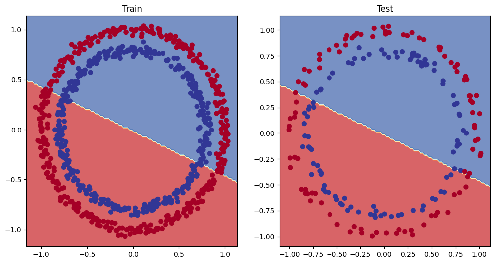
6. The missing piece: non-linearity
What patterns could you draw if you were given an infinite amount of a straight and non-straight lines?
Or in machine learning terms, an infinite (but really it is finite) linear and non-linear functions?
### 6.1 Recreating non-linear data(red and blue circles)

import matplotlib.pyplot as plt
from sklearn.datasets import make_circles

n_samples = 1000
X, y = make_circles(n_samples,
                    noise=0.03,
                   random_state=42)
plt.scatter(X[:, 0], X[:, 1], c=y, cmap=plt.cm.RdYlBu)
<matplotlib.collections.PathCollection at 0x7f956c226530>
# Convert data to tensors and train and test splits
import torch
from sklearn.model_selection import train_test_split

X = torch.from_numpy(X).type(torch.float)
y = torch.from_numpy(y).type(torch.float)

# Split into train and test
X_train, X_test, y_train, y_test = train_test_split(X,
                                                   y,
                                                   test_size=0.2,
random_state=42)X_train[:5], y_train[:5](tensor([[ 0.6579, -0.4651],
[ 0.6319, -0.7347],
[-1.0086, -0.1240],
[-0.9666, -0.2256],
[-0.1666, 0.7994]]),
tensor([1., 0., 0., 0., 1.]))6.2 Building a model with non-linearity
- Linear = straight lines
- Non-linear = non-straight lines
# Build a model with non-linear activation function
from torch import nn

class CircleModelV2(nn.Module):
    def __init__(self):
        super().__init__()
        self.layer_1 = nn.Linear(in_features=2, out_features=10)
        self.layer_2 = nn.Linear(in_features=10, out_features=10)
        self.layer_3 = nn.Linear(in_features=10, out_features=1)
        self.relu = nn.ReLU()

    def forward(self, x):
        return self.layer_3(self.relu(self.layer_2(self.relu(self.layer_1(x)))))

model_3 = CircleModelV2().to(device)
model_3
CircleModelV2(
(layer_1): Linear(in_features=2, out_features=10, bias=True)
(layer_2): Linear(in_features=10, out_features=10, bias=True)
(layer_3): Linear(in_features=10, out_features=1, bias=True)
(relu): ReLU()
)loss_fn = torch.nn.BCEWithLogitsLoss()
optimizer = torch.optim.SGD(params=model_3.parameters(), lr=0.1)torch.manual_seed(42)
torch.cuda.manual_seed(42)
epochs = 2500
X_train, y_train = X_train.to(device), y_train.to(device)
X_test, y_test = X_test.to(device), y_test.to(device)
for epoch in range(epochs):
model_3.train()
y_logits = model_3(X_train).squeeze()
loss = loss_fn(y_logits, y_train)
y_pred = torch.round(torch.sigmoid(y_logits))
acc = accuracy_fn(y_true=y_train, y_pred=y_pred)
optimizer.zero_grad()
loss.backward()
optimizer.step()
model_3.eval()
with torch.inference_mode():
y_test_logits = model_3(X_test).squeeze()
loss_test = loss_fn(y_test_logits, y_test)
y_test_pred = torch.round(torch.sigmoid(y_test_logits))
test_acc = accuracy_fn(y_true=y_test, y_pred=y_test_pred)
if epoch % 100 == 0:
print(f"epoch: {epoch}. Loss: {loss:.2f}. Accuracy: {acc:.2f}. Test Loss {loss_test:.2f}. Test accuracy: {test_acc:.2f}")epoch: 0. Loss: 0.69. Accuracy: 50.00. Test Loss 0.69. Test accuracy: 50.00
epoch: 100. Loss: 0.69. Accuracy: 52.88. Test Loss 0.69. Test accuracy: 52.50
epoch: 200. Loss: 0.69. Accuracy: 53.37. Test Loss 0.69. Test accuracy: 55.00
epoch: 300. Loss: 0.69. Accuracy: 53.00. Test Loss 0.69. Test accuracy: 56.00
epoch: 400. Loss: 0.69. Accuracy: 52.75. Test Loss 0.68. Test accuracy: 56.50
epoch: 500. Loss: 0.68. Accuracy: 52.75. Test Loss 0.68. Test accuracy: 56.50
epoch: 600. Loss: 0.68. Accuracy: 54.50. Test Loss 0.67. Test accuracy: 56.00
epoch: 700. Loss: 0.67. Accuracy: 58.38. Test Loss 0.66. Test accuracy: 59.00
epoch: 800. Loss: 0.65. Accuracy: 64.00. Test Loss 0.65. Test accuracy: 67.50
epoch: 900. Loss: 0.62. Accuracy: 74.00. Test Loss 0.62. Test accuracy: 79.00
epoch: 1000. Loss: 0.57. Accuracy: 87.75. Test Loss 0.57. Test accuracy: 86.50
epoch: 1100. Loss: 0.48. Accuracy: 93.50. Test Loss 0.50. Test accuracy: 90.50
epoch: 1200. Loss: 0.37. Accuracy: 97.75. Test Loss 0.41. Test accuracy: 92.00
epoch: 1300. Loss: 0.25. Accuracy: 99.00. Test Loss 0.30. Test accuracy: 96.50
epoch: 1400. Loss: 0.17. Accuracy: 99.50. Test Loss 0.22. Test accuracy: 97.50
epoch: 1500. Loss: 0.12. Accuracy: 99.62. Test Loss 0.17. Test accuracy: 99.00
epoch: 1600. Loss: 0.09. Accuracy: 99.88. Test Loss 0.13. Test accuracy: 99.50
epoch: 1700. Loss: 0.07. Accuracy: 99.88. Test Loss 0.10. Test accuracy: 99.50
epoch: 1800. Loss: 0.06. Accuracy: 99.88. Test Loss 0.09. Test accuracy: 99.50
epoch: 1900. Loss: 0.05. Accuracy: 99.88. Test Loss 0.07. Test accuracy: 99.50
epoch: 2000. Loss: 0.04. Accuracy: 99.88. Test Loss 0.07. Test accuracy: 100.00
epoch: 2100. Loss: 0.04. Accuracy: 99.88. Test Loss 0.06. Test accuracy: 100.00
epoch: 2200. Loss: 0.03. Accuracy: 99.88. Test Loss 0.05. Test accuracy: 100.00
epoch: 2300. Loss: 0.03. Accuracy: 99.88. Test Loss 0.05. Test accuracy: 100.00
epoch: 2400. Loss: 0.03. Accuracy: 99.88. Test Loss 0.05. Test accuracy: 100.00
# Plot decision boundary of the model
plt.figure(figsize=(12, 6))
plt.subplot(1, 2, 1)
plt.title("Train")
plot_decision_boundary(model_3, X_train, y_train)
plt.subplot(1, 2, 2)
plt.title("Test")
plot_decision_boundary(model_3, X_test, y_test)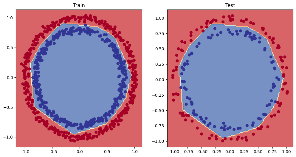
# make predictions
X_train, y_train = X_train.to("cpu"), y_train.to("cpu")
X_test, y_test = X_test.to("cpu"), y_test.to("cpu")

model_3.eval()
with torch.inference_mode():
    y_preds = torch.round(torch.sigmoid(model_3(X_test))).squeeze()

y_preds[:10], y_test[:10]
(tensor([1., 0., 1., 0., 1., 1., 0., 0., 1., 0.]),
tensor([1., 0., 1., 0., 1., 1., 0., 0., 1., 0.]))7. Replication non-linear activation functions
Neural networks, rather than us telling the model what to learn, we give it the tools to discover patterns in data and it tries to figure out the patterns on its own.
And these tools are linear & non-linear functions
# Create a tensor
A = torch.arange(-10, 10, 1, dtype=torch.float32)
A.dtypetorch.float32# Visualize the data
plt.plot(A)[<matplotlib.lines.Line2D at 0x7f956c3aab30>]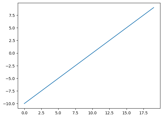
plt.plot(torch.relu(A))[<matplotlib.lines.Line2D at 0x7f956c0e3dc0>]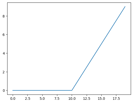
def relu(x: torch.Tensor) -> torch.Tensor:
    return torch.maximum(torch.tensor(0), x) # inputs must be tensors

plt.plot(relu(A))
[<matplotlib.lines.Line2D at 0x7f956c17bc70>]
# Let's do same for sigmoid
def sigmoid(x):
return 1 / (1 + torch.exp(-x))plt.plot(torch.sigmoid(A))[<matplotlib.lines.Line2D at 0x7f9565b7cc40>]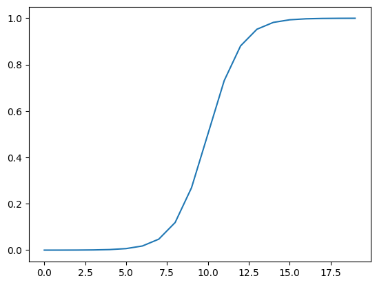
plt.plot(sigmoid(A))[<matplotlib.lines.Line2D at 0x7f9565c33940>]
8. Putting it all together with multi-class classification problem
- Binary classification = one thing or another(cat vs dog, spam vs not spam, fraud or not fraud)
- Multi-class classification = more than one thing or another(cat vs dog vs chichen)
import torch
import matplotlib.pyplot as plt
from sklearn.datasets import make_blobs
from sklearn.model_selection import train_test_split

# Set hyper parameters for data creation
NUM_CLASSES = 4
NUM_FEATURES = 2
RANDOM_SEED = 42

# 1. Create multi-class data
X_blob, y_blob = make_blobs(n_samples=1000,
                           n_features=NUM_FEATURES,
                           centers=NUM_CLASSES,
                           cluster_std=1.5,
                           random_state=RANDOM_SEED)
# 2. Turn data into tensors
X_blob = torch.from_numpy(X_blob).type(torch.float)
y_blob = torch.from_numpy(y_blob).type(torch.LongTensor)

# 3. Split into train and test
X_blob_train, X_blob_test, y_blob_train, y_blob_test = train_test_split(X_blob, y_blob, test_size=0.2, random_state=RANDOM_SEED)

# 4. Visualize
plt.figure(figsize=(10, 7))
plt.scatter(X_blob[:, 0], X_blob[:, 1], c=y_blob, cmap=plt.cm.RdYlBu)
<matplotlib.collections.PathCollection at 0x7f9565c31c30>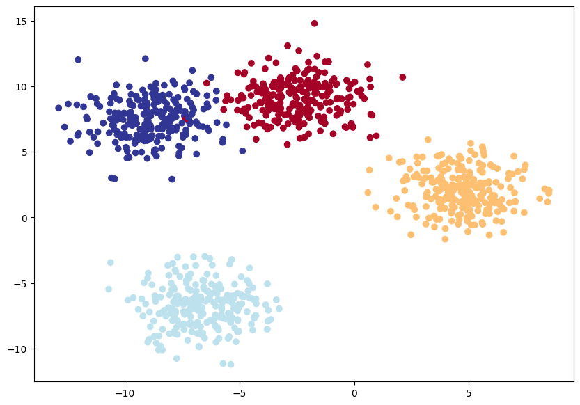
8.2 Building multiclass classification model in PyTorch
# Create device agnostic code
device = "cuda" if torch.cuda.is_available() else "cpu"
device'cuda'# Build multi-class classification model
class BlobModel(nn.Module):
def __init__(self, input_features, output_features, hidden_units=8):
"""
Initializes multi-class classification model.
Args:
input_features (int): Number of input features to the model
output_features (int): Number of output features (number of output classes)
hidden_units (int): Number of hidden units between layers, default 8
"""
super().__init__()
self.linear_layer_stack = nn.Sequential(
nn.Linear(in_features=input_features, out_features=hidden_units),
nn.ReLU(),
nn.Linear(in_features=hidden_units, out_features=hidden_units),
nn.ReLU(),
nn.Linear(in_features=hidden_units, out_features=output_features)
)
def forward(self, x):
return self.linear_layer_stack(x)
# Create an instance of blob model and send to target device
model_4 = BlobModel(input_features=2,
output_features=4,
hidden_units=8).to(device)
model_4BlobModel(
(linear_layer_stack): Sequential(
(0): Linear(in_features=2, out_features=8, bias=True)
(1): ReLU()
(2): Linear(in_features=8, out_features=8, bias=True)
(3): ReLU()
(4): Linear(in_features=8, out_features=4, bias=True)
)
)8.3 Create a loss function and an optimizer for a multi-class classification
# Create a loss function for multi-class classification
loss_fn = nn.CrossEntropyLoss()

optimizer = torch.optim.SGD(params=model_4.parameters(), lr=0.1)
8.4 Getting prediction probabilities for a multi-class PyTorch model
In order to evaluate and train our model, we need to convert our model outputs(logits) to prediction probabilities and then to prediction labels.
Logits (raw output of the model) -> Pred probs (use
torch.softmax) -> Pred labels (take the argmax of the
prediction probabilities)
model_4.eval()
with torch.inference_mode():
    y_logits = model_4(X_blob_test.to(device))[:5]

y_logits
tensor([[-0.7646, -0.7412, -1.5777, -1.1376],
[-0.0973, -0.9431, -0.5963, -0.1371],
[ 0.2528, -0.2379, 0.1882, -0.0066],
[-0.4134, -0.5204, -0.9303, -0.6963],
[-0.3118, -1.3736, -1.1991, -0.3834]], device='cuda:0')# Convert our model's logit output to prediction probabilities
y_pred_probs = torch.softmax(y_logits, dim=1)
y_pred_probs[:5]tensor([[0.3169, 0.3244, 0.1405, 0.2182],
[0.3336, 0.1432, 0.2026, 0.3206],
[0.3011, 0.1843, 0.2823, 0.2323],
[0.3078, 0.2766, 0.1836, 0.2320],
[0.3719, 0.1286, 0.1532, 0.3463]], device='cuda:0')torch.sum(y_pred_probs[0])tensor(1., device='cuda:0')torch.argmax(y_pred_probs[0])tensor(1, device='cuda:0')# Conver our model's prediction probabilities to prediction labels
y_preds = torch.argmax(y_pred_probs, dim=1)
y_predstensor([1, 0, 0, 0, 0], device='cuda:0')8.5 create a training and testing loop for a multi-class pytorch model
torch.manual_seed(42)
torch.cuda.manual_seed(42)
epochs = 100

X_blob_train, y_blob_train = X_blob_train.to(device), y_blob_train.to(device)
X_blob_test, y_blob_test = X_blob_test.to(device), y_blob_test.to(device)

for epoch in range(epochs):
    model_4.train()

    y_logits = model_4(X_blob_train)
    y_preds = torch.argmax(torch.softmax(y_logits, dim=1), dim=1)
    loss = loss_fn(y_logits, y_blob_train)
    acc = accuracy_fn(y_true=y_blob_train, y_pred=y_preds)

    optimizer.zero_grad()
    loss.backward()
    optimizer.step()

    model_4.eval()
    with torch.inference_mode():
        y_test_logits = model_4(X_blob_test)
        y_test_preds = torch.argmax(torch.softmax(y_test_logits, dim=1), dim=1)
        loss_test = loss_fn(y_test_logits, y_blob_test)
        acc_test = accuracy_fn(y_true=y_blob_test, y_pred=y_test_preds)

        if epoch % 10 == 0:
            print(f"Epoch {epoch} | Loss: {loss:.2f} | Accuracy: {acc:.2f} | Test loss: {loss_test:.2f} | Test Accuracy: {acc_test:.2f}")
Epoch 0 | Loss: 1.16 | Accuracy: 40.38 | Test loss: 1.08 | Test Accuracy: 48.00
Epoch 10 | Loss: 0.64 | Accuracy: 96.75 | Test loss: 0.66 | Test Accuracy: 97.50
Epoch 20 | Loss: 0.43 | Accuracy: 98.50 | Test loss: 0.43 | Test Accuracy: 100.00
Epoch 30 | Loss: 0.25 | Accuracy: 99.12 | Test loss: 0.25 | Test Accuracy: 99.50
Epoch 40 | Loss: 0.11 | Accuracy: 99.25 | Test loss: 0.10 | Test Accuracy: 99.50
Epoch 50 | Loss: 0.07 | Accuracy: 99.25 | Test loss: 0.06 | Test Accuracy: 99.50
Epoch 60 | Loss: 0.05 | Accuracy: 99.25 | Test loss: 0.04 | Test Accuracy: 99.50
Epoch 70 | Loss: 0.04 | Accuracy: 99.25 | Test loss: 0.03 | Test Accuracy: 99.50
Epoch 80 | Loss: 0.04 | Accuracy: 99.25 | Test loss: 0.03 | Test Accuracy: 99.50
Epoch 90 | Loss: 0.04 | Accuracy: 99.25 | Test loss: 0.03 | Test Accuracy: 99.50
8.6 Making and evaluating predictions with a PyTorch multi-class model
# Make predictions
model_4.eval()
model_4.to(device)
with torch.inference_mode():
    y_logits = model_4(X_blob_test.to(device))
    y_preds = torch.softmax(y_logits, dim=1).argmax(dim=1)

y_preds[:10], y_blob_test[:10]
(tensor([1, 3, 2, 1, 0, 3, 2, 0, 2, 0], device='cuda:0'),
tensor([1, 3, 2, 1, 0, 3, 2, 0, 2, 0], device='cuda:0'))# Plot decision boundary of the model
plt.figure(figsize=(12, 6))
plt.subplot(1, 2, 1)
plt.title("Train")
plot_decision_boundary(model_4, X_blob_train, y_blob_train)
plt.subplot(1, 2, 2)
plt.title("Test")
plot_decision_boundary(model_4, X_blob_test, y_blob_test)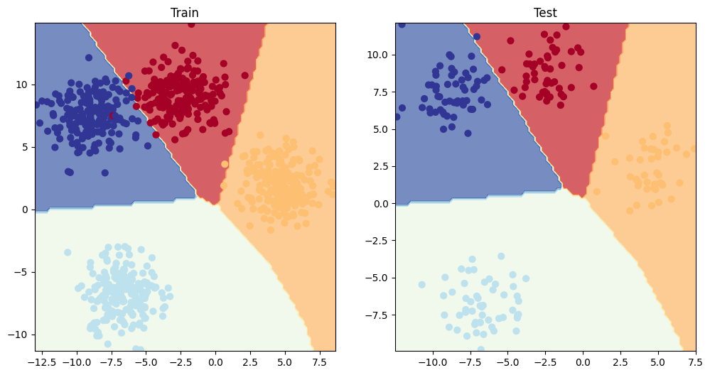
9. A few more classification metrics (to evaluate our classification model)
- Accuracy - out of 100 samples, how many does our model get right?
- Precision
- Recall
- F1-score
- Confusion matrix
- Classification report
See this article when to use precision and recall https://towardsdatascience.com/beyond-accuracy-precision-and-recall-3da06bea9f6c
import torchmetricsfrom torchmetrics import Accuracy
# Setup metric
torchmetric_accuracy = Accuracy(task='multiclass',
num_classes=NUM_CLASSES).to(device)
# Calculate accuracy
torchmetric_accuracy(y_preds, y_blob_test)tensor(0.9950, device='cuda:0')Excercises
- Make a binary classification dataset with Scikit-Learn's make_moons() function. For consistency, the dataset should have 1000 samples and a random_state=42. Turn the data into PyTorch tensors. Split the data into training and test sets using train_test_split with 80% training and 20% testing.
import torch
from torch import nn
from sklearn.datasets import make_moons
from sklearn.model_selection import train_test_split
moons_numpy = make_moons(n_samples=1000, random_state=42)
X, y = moons_numpy[0], moons_numpy[1]
X_train, X_test, y_train, y_test = train_test_split(X, y, test_size=0.2, random_state=42)device = "cuda" if torch.cuda.is_available() else "cpu"
device'cuda'X_train = torch.from_numpy(X_train).to(device).type(torch.float)
X_test = torch.from_numpy(X_test).to(device).type(torch.float)
y_train = torch.from_numpy(y_train).to(device).type(torch.float)
y_test = torch.from_numpy(y_test).to(device).type(torch.float)
len(X_train), len(y_train),len(X_test), len(y_test)(800, 800, 200, 200)- Build a model by subclassing nn.Module that incorporates non-linear activation functions and is capable of fitting the data you created in 1. Feel free to use any combination of PyTorch layers (linear and non-linear) you want.
# 2- Visualizing the dataset.
from matplotlib import pyplot as plt

# When the label y is 0, the class is represented with a blue square.
# When the label y is 1, the class is represented with a green triangle.
plt.plot(moons_numpy[0][:, 0][moons_numpy[1]==1], moons_numpy[0][:, 1][moons_numpy[1]==1], "bs")
plt.plot(moons_numpy[0][:, 0][moons_numpy[1]==0], moons_numpy[0][:, 1][moons_numpy[1]==0], "g^")

# X contains two features, x1 and x2
plt.xlabel(r"$x_1$", fontsize=20)
plt.ylabel(r"$x_2$", fontsize=20)

# Simplifying the plot by removing the axis scales.
plt.xticks([])
plt.yticks([])

# Displaying the plot.
plt.show()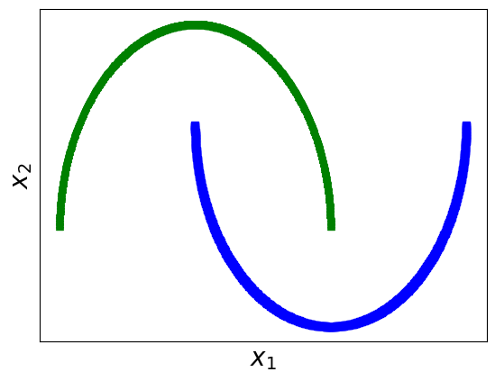
class MoonModel(nn.Module):
    def __init__(self):
        super().__init__()
        self.layers = nn.Sequential(
            nn.Linear(in_features=2, out_features=10),
            nn.ReLU(),
            nn.Linear(in_features=10, out_features=10),
            nn.ReLU(),
            nn.Linear(in_features=10, out_features=1)
        )

    def forward(self, x):
        return self.layers(x)

moon_model = MoonModel().to(device)
moon_model
MoonModel(
(layers): Sequential(
(0): Linear(in_features=2, out_features=10, bias=True)
(1): ReLU()
(2): Linear(in_features=10, out_features=10, bias=True)
(3): ReLU()
(4): Linear(in_features=10, out_features=1, bias=True)
)
)- Setup a binary classification compatible loss function and optimizer to use when training the model.
loss_fn = nn.BCEWithLogitsLoss()
optimizer = torch.optim.SGD(params = moon_model.parameters(), lr=0.1)- Create a training and testing loop to fit the model you created in 2 to the data you created in 1. To measure model accuray, you can create your own accuracy function or use the accuracy function in TorchMetrics. Train the model for long enough for it to reach over 96% accuracy. The training loop should output progress every 10 epochs of the model's training and test set loss and accuracy.
import torchmetrics

torch.manual_seed(42)
torch.cuda.manual_seed(42)

accuracy_fn = Accuracy(task='binary').to(device)

epochs = 810

for epoch in range(epochs):
    moon_model.train()

    y_logits = moon_model(X_train).squeeze()
    loss = loss_fn(y_logits, y_train)
    acc = accuracy_fn(torch.round(torch.sigmoid(y_logits)), y_train)
    optimizer.zero_grad()
    loss.backward()
    optimizer.step()

    moon_model.eval()
    y_test_logits = moon_model(X_test).squeeze()
    acc_test = accuracy_fn(torch.round(torch.sigmoid(y_test_logits)), y_test)
    loss_test = loss_fn(y_test_logits, y_test)

    if epoch % 100 == 0:
        print(f"Epoch: {epoch} | Loss {loss} | Accuracy {acc}| Test Loss {loss_test} | Test Accuracy {acc_test}")
Epoch: 0 | Loss 0.6953642964363098 | Accuracy 0.3725000023841858| Test Loss 0.6946236491203308 | Test Accuracy 0.5
Epoch: 100 | Loss 0.3858400583267212 | Accuracy 0.8162500262260437| Test Loss 0.40273696184158325 | Test Accuracy 0.7649999856948853
Epoch: 200 | Loss 0.23520521819591522 | Accuracy 0.887499988079071| Test Loss 0.23914630711078644 | Test Accuracy 0.9100000262260437
Epoch: 300 | Loss 0.18843956291675568 | Accuracy 0.9162499904632568| Test Loss 0.18707025051116943 | Test Accuracy 0.925000011920929
Epoch: 400 | Loss 0.14797131717205048 | Accuracy 0.9387500286102295| Test Loss 0.14572730660438538 | Test Accuracy 0.9399999976158142
Epoch: 500 | Loss 0.10224613547325134 | Accuracy 0.9612500071525574| Test Loss 0.09955348819494247 | Test Accuracy 0.9750000238418579
Epoch: 600 | Loss 0.06423261761665344 | Accuracy 0.987500011920929| Test Loss 0.06165194883942604 | Test Accuracy 0.9850000143051147
Epoch: 700 | Loss 0.04050951078534126 | Accuracy 1.0| Test Loss 0.038339946419000626 | Test Accuracy 1.0
Epoch: 800 | Loss 0.027203937992453575 | Accuracy 1.0| Test Loss 0.025386687368154526 | Test Accuracy 1.0
- Make predictions with your trained model and plot them using the plot_decision_boundary() function created in this notebook.
# Plot decision boundary of the model
plt.figure(figsize=(12, 6))
plt.subplot(1, 2, 1)
plt.title("Train")
plot_decision_boundary(moon_model, X_train, y_train)
plt.subplot(1, 2, 2)
plt.title("Test")
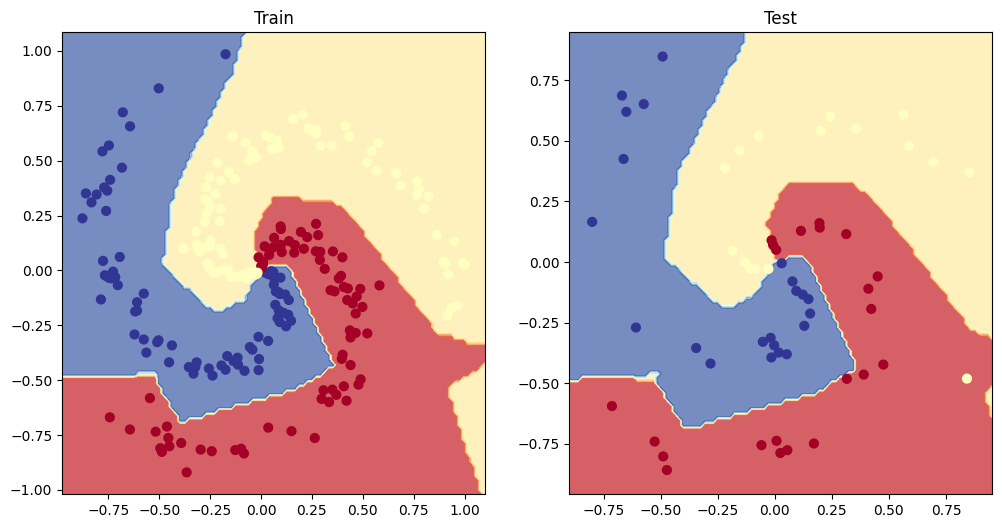
plot_decision_boundary(moon_model, X_test, y_test)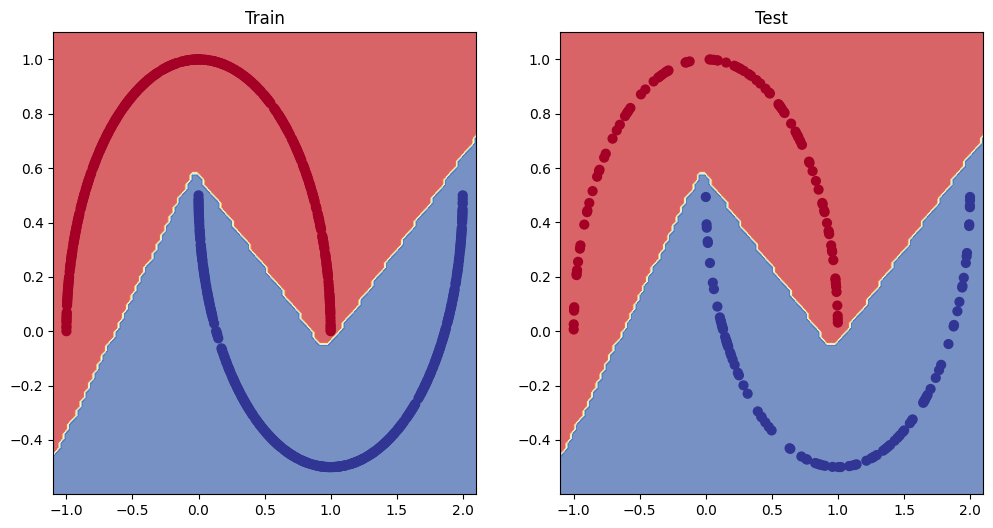
6.Replicate the Tanh (hyperbolic tangent) activation function in pure PyTorch. Feel free to reference the ML cheatsheet website for the formula.
def tanh(z):
return (torch.exp(z) - torch.exp(-z)) / (torch.exp(z) + torch.exp(-z))- Create a multi-class dataset using the spirals data creation function from CS231n (see below for the code). Construct a model capable of fitting the data (you may need a combination of linear and non-linear layers). Build a loss function and optimizer capable of handling multi-class data (optional extension: use the Adam optimizer instead of SGD, you may have to experiment with different values of the learning rate to get it working). Make a training and testing loop for the multi-class data and train a model on it to reach over 95% testing accuracy (you can use any accuracy measuring function here that you like). Plot the decision boundaries on the spirals dataset from your model predictions, the plot_decision_boundary() function should work for this dataset too.
# Code for creating a spiral dataset from CS231n
import numpy as np
N = 100 # number of points per class
D = 2 # dimensionality
K = 3 # number of classes
X = np.zeros((N*K,D)) # data matrix (each row = single example)
y = np.zeros(N*K, dtype='uint8') # class labels
for j in range(K):
  ix = range(N*j,N*(j+1))
  r = np.linspace(0.0,1,N) # radius
  t = np.linspace(j*4,(j+1)*4,N) + np.random.randn(N)*0.2 # theta
  X[ix] = np.c_[r*np.sin(t), r*np.cos(t)]
  y[ix] = j
# lets visualize the data
plt.scatter(X[:, 0], X[:, 1], c=y, s=40, cmap=plt.cm.Spectral)
plt.show()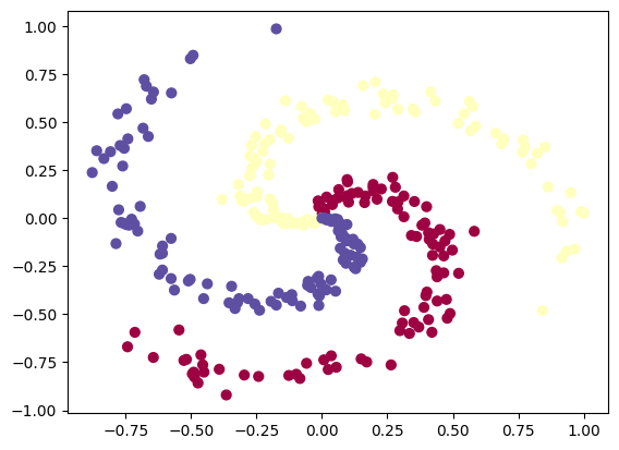
len(X), len(y)(300, 300)X_train, X_test, y_train, y_test = train_test_split(X, y, test_size=0.2, random_state=42)
X_train = torch.from_numpy(X_train).type(torch.float).to(device)
X_test = torch.from_numpy(X_test).type(torch.float).to(device)
y_train = torch.from_numpy(y_train).type(torch.torch.LongTensor).to(device)
y_test = torch.from_numpy(y_test).type(torch.torch.LongTensor).to(device)
print(len(X_train), len(y_train),len(X_test), len(y_test))
print(X_train.device, y_train.device, X_test.device, y_test.device)240 240 60 60
cuda:0 cuda:0 cuda:0 cuda:0
class SpiralModel(nn.Module):
    def __init__(self):
        super().__init__()
        self.layers = nn.Sequential(
            nn.Linear(in_features=2, out_features=10),
            nn.ReLU(),
            nn.Linear(in_features=10, out_features=10),
            nn.ReLU(),
            nn.Linear(in_features=10, out_features=3)
        )

    def forward(self, x):
        return self.layers(x)

spiral_model = SpiralModel().to(device)
spiral_model
SpiralModel(
(layers): Sequential(
(0): Linear(in_features=2, out_features=10, bias=True)
(1): ReLU()
(2): Linear(in_features=10, out_features=10, bias=True)
(3): ReLU()
(4): Linear(in_features=10, out_features=3, bias=True)
)
)loss_fn = nn.CrossEntropyLoss()
optimizer = torch.optim.SGD(params = spiral_model.parameters(), lr=0.01)import torchmetrics
torch.manual_seed(42)
torch.cuda.manual_seed(42)
accuracy_fn = Accuracy(task='multiclass', num_classes=3).to(device)
epochs = 60001
for epoch in range(epochs):
moon_model.train()
y_logits = spiral_model(X_train)
loss = loss_fn(y_logits, y_train.to(device))
acc = accuracy_fn(torch.softmax(y_logits, dim=1).argmax(dim=1), y_train)
optimizer.zero_grad()
loss.backward()
optimizer.step()
moon_model.eval()
y_test_logits = spiral_model(X_test)
acc_test = accuracy_fn(torch.softmax(y_test_logits, dim=1).argmax(dim=1), y_test)
loss_test = loss_fn(y_test_logits, y_test)
if epoch % 10000 == 0:
print(f"Epoch: {epoch} | Loss {loss:.2f} | Accuracy {acc:.2f}| Test Loss {loss_test:.2f} | Test Accuracy {acc_test:.2f}")Epoch: 0 | Loss 1.12 | Accuracy 0.32| Test Loss 1.11 | Test Accuracy 0.37
Epoch: 10000 | Loss 0.54 | Accuracy 0.70| Test Loss 0.67 | Test Accuracy 0.63
Epoch: 20000 | Loss 0.26 | Accuracy 0.93| Test Loss 0.28 | Test Accuracy 0.92
Epoch: 30000 | Loss 0.13 | Accuracy 0.97| Test Loss 0.15 | Test Accuracy 0.93
Epoch: 40000 | Loss 0.08 | Accuracy 0.98| Test Loss 0.12 | Test Accuracy 0.93
Epoch: 50000 | Loss 0.06 | Accuracy 0.98| Test Loss 0.11 | Test Accuracy 0.97
Epoch: 60000 | Loss 0.05 | Accuracy 0.99| Test Loss 0.09 | Test Accuracy 0.98
# Plot decision boundary of the model
plt.figure(figsize=(12, 6))
plt.subplot(1, 2, 1)
plt.title("Train")
plot_decision_boundary(spiral_model, X_train, y_train)
plt.subplot(1, 2, 2)
plt.title("Test")
plot_decision_boundary(spiral_model, X_test, y_test)